How to plan a cervical spine MRI protocol

This step-by-step guide is for MRI students, radiographers, and technologists who wish to improve their planning skills and master the cervical spine MRI protocol.

What you will learn:

1. Key factors in cervical spine MRIs, including trade-offs.
2. Patient and scanner setup tips.
3. Best pulse sequences and planning techniques.
4. Ways to avoid common artifacts.
5. What great cervical spine images should look like.

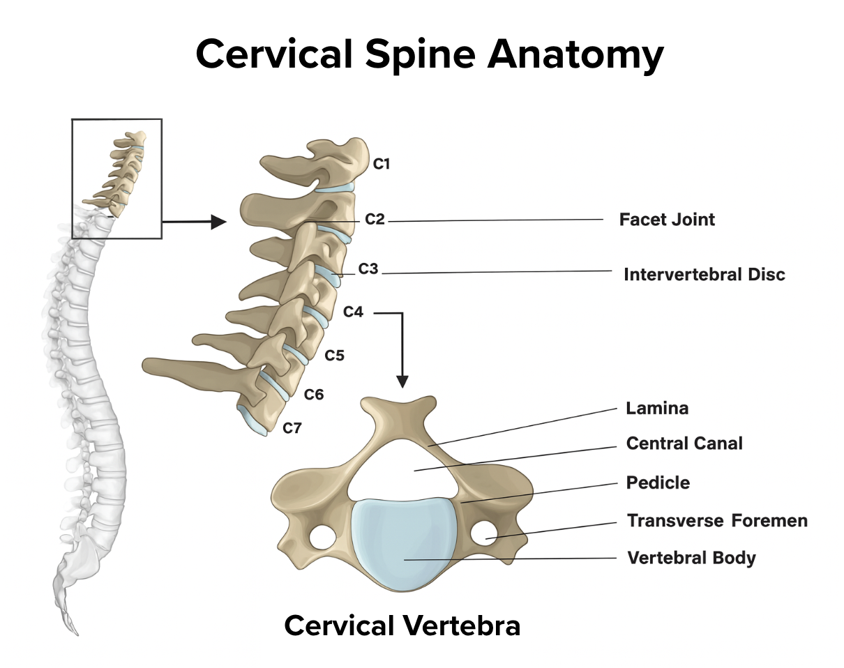
The cervical spine consists of seven vertebrae (C1–C7) that support the head and protect the spinal cord in the neck region. This area is highly mobile and vulnerable to injury from trauma, degenerative changes, and various pathological processes.

Because of its central role in supporting the head and protecting vital neural structures, the cervical spine is one of the most frequently examined areas in MRI. Imaging helps assess disc herniation, spinal stenosis, cord compression, traumatic injuries, and other conditions that can significantly impact neurological function and quality of life.

How to Balance the 3 Trade-offs in Cervical Spine MRIs

In MRI, we always face a trade-off between 3 key metrics:

• Scan Time: How fast a pulse sequence can be completed.
• Resolution: How much detail the image can display.
• SNR: How clear the image is, meaning how much signal we have compared with noise.

Improving one of these metrics often reduces the performance of the others. To decide what trade-offs to make, we must consider the needs of each clinical situation.

For cervical spine MRIs, we face these challenges:

• The structures we are looking for are small. Disc protrusions, nerve root compression and early cord signal change can measure only a few millimeters, so without high in-plane resolution we can miss them.
• The diagnosis rests on contrast between four tissues that sit directly against each other: spinal cord, cerebrospinal fluid, disc material and nerve roots. Smaller voxels lower SNR, so enough signal has to be left to keep those borders distinct.
• The neck moves and the fluid around the cord pulsates. Swallowing and CSF flow both produce ghosting along the phase direction, and a longer acquisition gives both more opportunity to blur the detail we are trying to resolve.

Therefore, we typically:

1. Slightly prioritize resolution to show small disc protrusions, foraminal narrowing and early cord compression.
2. Maintain good enough SNR to keep the borders between cord, CSF and disc material distinct.
3. Optimize scan time last, keeping it short enough that swallowing and CSF flow do not blur the resolution we paid for.

Cervical Spine Health Conditions and the MRI Sequences That Reveal Them

1.5 T vs 3 T – What Changes at Higher Field Strengths?

This guide demonstrates the protocol at 3 T, with a dedicated comparison against 1.5 T in this section. With the exception of the 1.5 T comparison image below, all example images are acquired at 3 T to show the image quality achievable with higher field strength.

When we move from 1.5 T to 3 T, three important things change:

1. Signal Increases and Priorities Change

At 3 T, we gain a substantial increase in signal compared with 1.5 T, though less than the doubling that field strength alone would suggest.

Since we now have more signal than this protocol needs at baseline, SNR drops to third priority. We can invest the extra signal to either increase resolution (see finer details) or reduce scan time while maintaining the same quality.

For cervical spine imaging, we typically invest this signal gain into improved resolution to better visualize fine anatomical structures like small disc herniations and nerve root compression.

2. Frequency Precession Differences Double

The frequency precession difference between fat and water spins doubles from ~220 Hz at 1.5 T to ~440 Hz at 3 T.

This means we must increase our bandwidth per pixel to around 440 Hz to prevent chemical shift artifacts.

3. T1 Relaxation Times Are Prolonged

At higher magnetic field strengths, most tissues (including fat) have longer T1 relaxation times. This means it takes longer for magnetization to recover after an inversion pulse.

This specifically affects STIR sequences, which use an inversion recovery pulse to null fat signal. The TI must be timed to catch fat magnetization at the exact moment it crosses zero (null point).

Since fat takes longer to relax at 3 T, we need a longer TI (around 180–220 ms) to hit that null point. If we used the TI value for 1.5 T at 3 T also, we'd null the fat too early and get incomplete fat suppression.

Key Parameter Adjustments for 3 T

These values apply to the sagittal and coronal sequences. The axial sequences use a smaller field of view and matrix, a larger slice gap and a lower bandwidth, and the STIR uses its own bandwidth and timing.

1.5 T vs 3 T – Image Quality Comparison

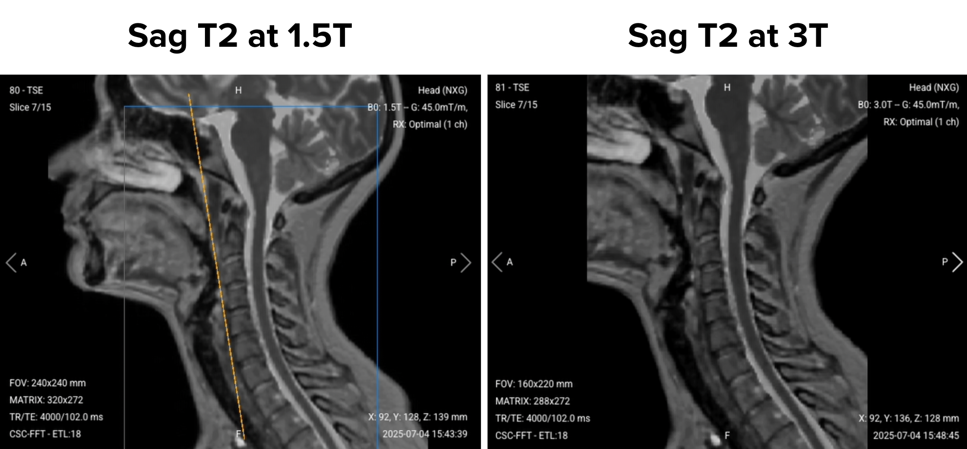
The images below show sagittal T2 TSE sequences acquired at both field strengths, demonstrating the resolution and scan time improvements achievable at 3 T:

What parameters were used to acquire the above images:

The result of each acquisition:

Key Improvements at 3 T:

1. Better resolution: 31% smaller voxel volume reveals finer anatomical details
2. Faster scanning: 50% reduction in scan time improves patient comfort and workflow
3. Signal reinvested: SNR is lower because signal was traded for smaller voxels and a shorter scan.

3 T lets us invest the signal gain into resolution and a shorter scan, at the cost of lower SNR.

The step-by-step guide below will show you how to set up and perform a cervical spine MRI protocol in practice.

We will perform the protocol in 3 parts:

1. Set up the Patient and MRI Scanner
2. Plan and Acquire the Protocol Sequences
3. Review the Images

Part 1: Set up the Patient and MRI Scanner

1. Position the Patient in the Scanner

Lay the patient head-first and supine (on their back) with the head and neck centered at the scanner's isocenter.

The positioning for cervical spine examinations is similar to how we position a patient for neuro examinations, as we use the same coil system.

Use a dedicated brain coil with extension to ensure high-resolution imaging. The brain coil offers an extension that goes from the vertex of the head down to the cervical spine segment, providing strong signal reception and full coverage of the cervical region.

✅ Correct Patient Positioning:

2. Check the Scanner's Hardware Settings

Once the patient is in place, review your scanner's hardware settings.

In this guide, we will use the following settings:

This hardware setup is widely used in clinical practice. It balances acquisition time, image quality, and patient comfort.

3. Capture the Initial Localizer Images

Before we can perform any MRI protocol, we must always capture initial localizer images of the patient. These images act as a guide for planning the detailed scans we will perform next.

We should always capture localizers in three planes:

1. Axial
2. Sagittal
3. Coronal

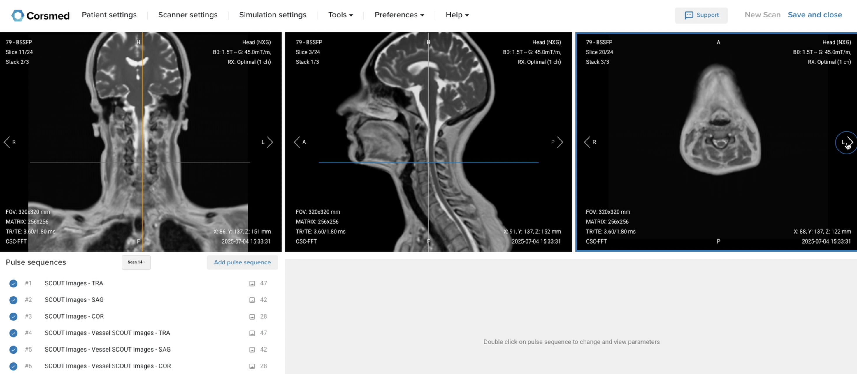
Once acquired, load the initial localizer images into the three viewports.

Then, scroll through each of the image stacks to locate a central slice that clearly shows the anatomy of the cervical spine.

✅ Correct Setup of Localizer Images for Cervical Spine MRI:

Part 2: Plan and Acquire the Protocol Sequences

When all preparations are ready, we can start planning and acquiring the protocol sequences.

Let's go through the pulse sequences a standard cervical spine MRI protocol includes, why we perform them, and how to set them up.

The 6 Sequences of a Standard Cervical Spine MRI Protocol

1. Sagittal T2 TSE
2. Sagittal T1 TSE
3. Sagittal STIR TSE
4. Coronal T2 TSE
5. Axial T2 TSE
6. Axial T1 TSE

We mainly use Turbo/Fast Spin Echo sequences for this study. These sequences provide fast, high-quality images with excellent soft tissue contrast and minimal artifacts, making them ideal for cervical spine diagnosis.

Turbo Spin Echo also lets us create multiple types of contrasts, including T2, T1, and inversion recovery for fat suppression. This helps us assess the spine's structure, detect abnormalities, and identify common pathologies like disc herniation, cord compression, and inflammation.

This sequence selection is a common standard rather than a fixed rule. Always confirm that your protocol matches the requirements of your own department, and note that accreditation bodies may specify sequence types and coverage that differ from a routine clinical protocol.

The values in the tables below are worked examples for the 3 T setup used in this guide. Exact numbers vary by scanner, coil and department, so treat them as a starting point rather than as fixed limits.

In the sections below, we go through how to plan and set up each sequence.

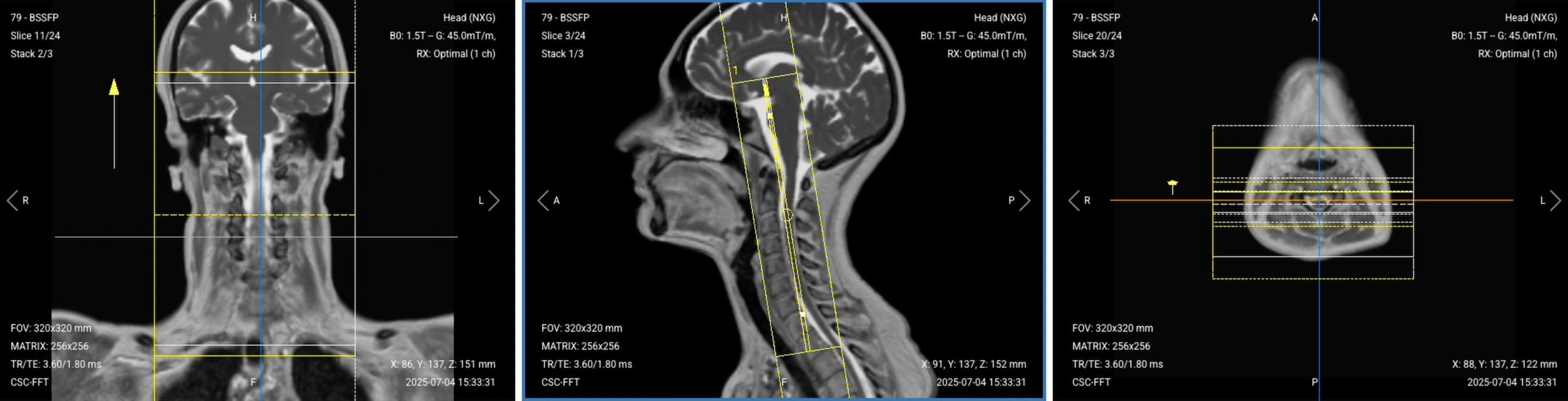
1. Planning Sagittal T2 TSE

✅ Correct Planning:

Planning Instructions:

• Use the spinal cord as your anatomical reference.
• Align the slices as follows:
  • Coronal localizer: Grab the slice and align it parallel to the spinal cord direction.
  • Axial localizer: Ensure the line passes through the middle of the vertebral body, following all the way back to the posterior processes of the vertebrae.
• Use appropriate geometry parameters:
  • Slice number: Enough to cover vertebral bodies from right to left (typically 15–20 slices).
  • Slice thickness: 3 mm, thin enough to resolve disc margins and nerve root compression.
  • Slice gap: 0.3 mm, 10% of slice thickness, which limits cross-talk without hiding anatomy.
• Set the foldover direction (phase encoding) to foot-to-head (FH) to align with CSF flow direction and minimize flow artifacts.

Parameters for Sagittal T2 TSE:

2. Planning Sagittal T1 TSE

✅ Correct Planning:

Planning Instructions:

• Copy the slice geometry and planning from the previous sagittal T2 sequence.
• Keep the same slice angulation, coverage, and positioning to ensure images of different contrasts can be clearly compared.

Parameters for Sagittal T1 TSE:

3. Planning Sagittal STIR TSE

✅ Correct Planning:

Planning Instructions:

• Copy the slice geometry and planning from the previous sagittal T1 sequence.
• Keep the same slice angulation, coverage, and positioning to ensure images of different contrasts can be clearly compared.

Parameters for Sagittal STIR TSE:

4. Planning Coronal T2 TSE

✅ Correct Planning:

Planning Instructions:

• Use the spinal cord as your anatomical reference.
• Align the slices as follows:
  • Sagittal localizer: Align slices parallel to the spine and center them.
  • Axial localizer: Slices should be perpendicular to the midline that passes through the vertebral body to the posterior processes.
• Use appropriate geometry parameters:
  • Slice number: Enough to cover from anterior cervical spine to posterior (typically 15–25 slices).
  • Slice thickness: 3 mm, consistent with sagittal sequences.
  • Slice gap: 0.3 mm, maintains consistency with other sequences.
• Set the foldover direction (phase encoding) to foot-to-head (FH) to avoid flow artifacts, same as sagittal sequences.

Parameters for Coronal T2 TSE:

5. Planning Axial T2 TSE

✅ Correct Planning:

Planning Instructions:

• Use the cervical spine and intervertebral discs as your anatomical references.
• Align the slices as follows:
  • Sagittal localizer: Slices should be perpendicular to the cervical spine.
  • Coronal localizer: Slices should run parallel to the intervertebral spaces.
• Use appropriate geometry parameters:
  • Slice number: Enough to cover C1–C7 and their discs, typically 30–35 slices.
  • Slice thickness: 3 mm, same as other sequences.
  • Slice gap: 1 mm, wider than on the sagittal sequences to extend coverage.
• Set the foldover direction (phase encoding) to anterior-posterior (AP) to align with the axial anatomy shape.
• Place a saturation band on the patient's throat to suppress swallowing artifacts without covering the cervical discs.

Parameters for Axial T2 TSE:

6. Planning Axial T1 TSE

✅ Correct Planning:

Planning Instructions:

• Copy the slice geometry and planning from the previous axial T2 sequence.
• Keep the same slice angulation, coverage, and positioning to ensure images of different contrasts can be clearly compared.
• Keep the same saturation band placement on the throat.

Parameters for Axial T1 TSE:

How to Avoid Artifacts When Planning the Sequences

The table below lists the 5 common cervical spine artifacts, and what techniques you can use to avoid them:

Part 3: Review the Images

Finally, we will review the images to ensure all the anatomical information we need is clear.

These key structures must be clearly visible in a cervical spine MRI:

1. Spinal cord and central canal
2. Cerebrospinal fluid spaces
3. Intervertebral discs (C2–C3 through C7–T1)
4. Vertebral bodies (C1–C7 and T1–T2)
5. Neural foramina and nerve roots
6. Ligamentous structures
7. Surrounding soft tissues

Below, we will go through all the different image contrasts and explain their specific role in imaging the cervical spine.

T2 TSE – Highlights Fluid-Related Tissues and Conditions

T2-weighted imaging makes fluids appear bright. This contrast is ideal for tissues and abnormalities with high water content.

In cervical spine MRI, T2 sequences are the gold standard for detecting spinal cord compression, disc herniation, myelopathy, and cord edema. The bright cerebrospinal fluid provides excellent contrast against the darker spinal cord, making compression visible as narrowing of the bright CSF space around the cord.

We capture T2 images in three planes (sagittal, coronal, and axial) to provide comprehensive visualization of spinal pathology from multiple angles.

✅ Sagittal T2 TSE of the Cervical Spine – Correct Image Example:

Things to Look for in Sagittal T2:

• Bright CSF should surround the dark spinal cord without narrowing.
• Intervertebral discs should show normal hydration (bright signal).
• Look for disc herniations compressing the thecal sac.
• Assess for cord signal changes indicating myelopathy.

✅ Coronal T2 TSE of the Cervical Spine – Correct Image Example:

Things to Look for in Coronal T2:

• Neural foramina should be open and symmetric.
• Look for lateral disc herniations or foraminal stenosis.
• Assess spinal cord alignment and any lateral compression.

✅ Axial T2 TSE of the Cervical Spine – Correct Image Example:

Things to Look for in Axial T2:

• Central canal should be patent with bright CSF.
• Disc material should not indent the thecal sac.
• Neural foramina should be symmetric and uncompressed.
• Look for any soft tissue masses or ligamentum flavum hypertrophy.

STIR TSE – Clearest View of Fluid-Related Tissues and Conditions

STIR (Short TI Inversion Recovery) suppresses fat signals completely, which makes water-rich tissues stand out even clearer than with normal T2 TSE. This makes STIR ideal for detecting subtle fluid-related conditions such as edema, inflammation, and infections, where increased water content would otherwise be obscured by fat.

In the cervical spine, this contrast is particularly useful for identifying bone marrow edema, ligament tears, cord contusions, and infections like discitis or myelitis. STIR is the key sequence for detecting acute trauma injuries and inflammatory conditions where water content might not be visible on standard T2 sequences.

We capture STIR images in the sagittal plane to provide comprehensive assessment of inflammatory and traumatic changes.

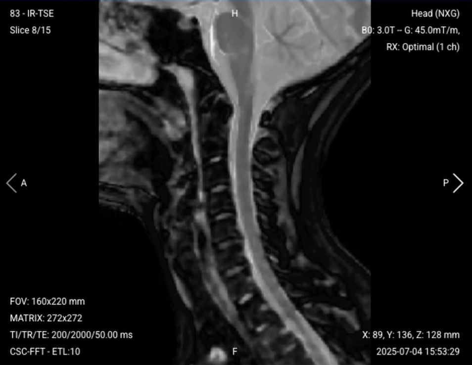
✅ Sagittal STIR TSE of the Cervical Spine – Correct Image Example:

Things to Look for in Sagittal STIR:

• Fat should appear uniformly dark (well-suppressed).
• Look for bright signal in bones indicating marrow edema.
• Assess ligaments for tears or inflammation.
• Look for any inflammatory processes in soft tissues.
• Evaluate for cord edema or contusion.

T1 TSE – Highlights Fat-Containing Tissues and Structural Abnormalities

T1-weighted imaging makes fat appear bright and fluid dark. This contrast is ideal for fat-rich tissues and structural abnormalities. T1 shows anatomical structures clearly, since it helps us see where different solid tissues like muscle and fat meet.

In cervical spine MRI, T1 sequences are important for evaluating vertebral body integrity, bone marrow pathology, and anatomical landmarks. T1 is also useful for detecting subacute hemorrhage, tumors, and serves as a baseline before contrast administration.

We capture T1 images in sagittal and axial planes to provide structural detail complementary to the T2 sequences.

✅ Sagittal T1 TSE of the Cervical Spine – Correct Image Example:

Things to Look for in Sagittal T1:

• Vertebral bodies should show bright, uniform bone marrow signal.
• Look for dark lesions indicating metastases or fractures.
• Assess disc height and alignment.
• Evaluate pre-vertebral soft tissues for masses or swelling.

✅ Axial T1 TSE of the Cervical Spine – Correct Image Example:

Things to Look for in Axial T1:

• Bone marrow should appear bright and symmetric.
• Look for fat-containing lesions like lipomas.
• Assess vertebral body structural integrity.
• Evaluate surrounding soft tissue anatomy.

Final Checks:

Before finishing a cervical spine MRI, always check these 5 points to ensure diagnostic quality:

1. Complete Coverage: Sagittal sequences must cover from the pons to T1–T2. Coronal and axial sequences must cover all seven cervical vertebrae and their discs, with coronal covering from the anterior vertebral bodies through to the posterior elements, and axial covering all seven cervical vertebrae and their discs.
2. Spinal Cord Visibility: The spinal cord and CSF spaces must be clearly visible throughout the cervical region in all sequences.
3. Image Quality: All images must have strong SNR, sharp anatomical detail, and no significant motion, flow, or chemical shift artifacts.
4. Consistent Planning: Sagittal, coronal, and axial planes must be properly aligned to the spinal anatomy for accurate assessment.
5. Artifact Management: Check that saturation bands are properly placed, foldover suppression is active, and bandwidth is optimized for the field strength.

‍