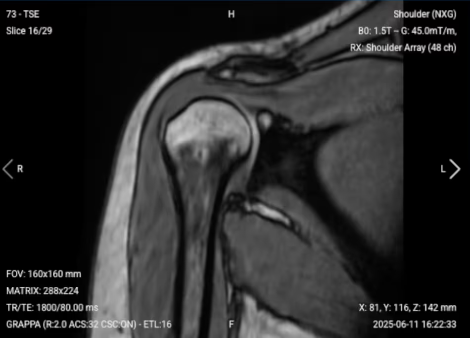
How to plan a shoulder MRI protocol (clock face method)
Written by:
Erik Jacobsson
This step-by-step guide is for MRI students, radiographers, and technologists who wish to improve their planning skills and master the shoulder MRI protocol.
What you will learn:
Key factors in shoulder MRIs, including trade-offs.
Patient and scanner setup tips.
Best pulse sequences and planning techniques.
Ways to avoid common artifacts.
What great shoulder images should look like.
Key Takeaways
Because shoulder MRIs require high detail for small structures, it's recommended to prioritize resolution.
The shoulder contains fine structures like the labrum, rotator cuff tendons, and cartilage that need high resolution to detect subtle tears and pathologies.
We should therefore 1) prioritize resolution, 2) maintain strong SNR for clarity, and 3) optimize scan time as needed.
We mainly use PD Fat-Saturated sequences in shoulder MRIs.
PD FS sequences offer excellent soft tissue contrast and highlight fluids while suppressing fat signal. This helps us clearly see ligament and tendon tears, labral issues, and bone marrow edema.
Fat suppression avoids interference, so these sequences are ideal for evaluating soft tissues in the shoulder.
Avoid these 5 common shoulder artifacts.
Artifacts
Solution – How to Avoid It
Motion artifacts
Shorten the scan time to reduce the risk of patient movement.
Magic angle artifacts
Acquire T2-weighted images to check if the signal is artifact or real tendon pathology.
Chemical shift artifacts
Increase the bandwidth to reduce spatial shift between fat and water signals.
Wrap-around artifacts
Activate fold-over suppression to block signals from anatomy outside the field of view.
Susceptibility artifacts
Use spin echo sequences instead of gradient echo sequences.
Cross-talk artifacts
Keep enough slice gap to prevent overlap between slices.
Intro to Shoulder MRIs
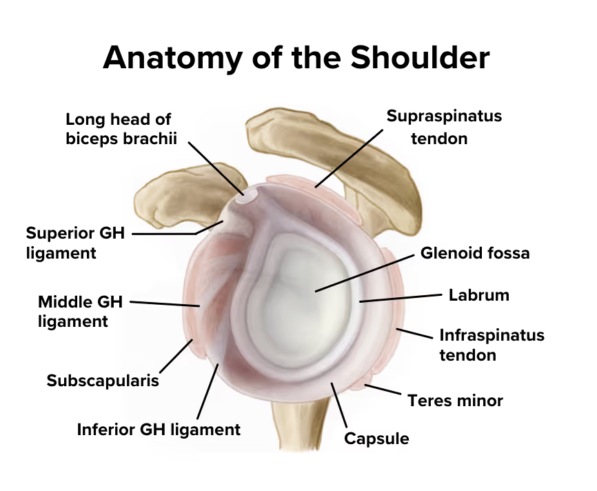
The shoulder is a complex ball-and-socket joint that enables the widest range of motion of any joint in the human body. It consists of multiple structures including the rotator cuff tendons, labrum, joint capsule, and surrounding muscles that work together to provide both mobility and stability.
Because of its complex anatomy and high susceptibility to injuries from sports, repetitive use, and trauma, the shoulder is a frequently examined area in MRI. Imaging helps assess rotator cuff tears, labral damage, impingement syndromes, and other conditions affecting shoulder function and causing pain.
How to Balance the 3 Trade-offs in Shoulder MRIs
In MRI, we always face a trade-off between 3 key metrics:
Scan Time: How fast a pulse sequence can be completed.
Resolution: How much detail the image can display.
SNR: How clear the image is, how much signal relative to noise.
Improving one of these metrics reduces the performance of the others. To decide what trade-offs to make, we must consider the needs of each clinical situation.
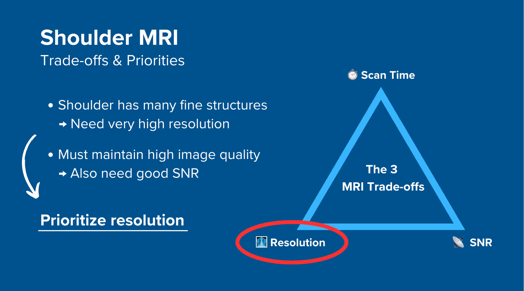
In shoulder MRIs, we have many fine structures like the labrum, rotator cuff tendons, and cartilage. These require very high resolution to detect subtle tears and pathologies. However, this high resolution reduces SNR, so to maintain image clarity, we must compensate with strong SNR.
Therefore, we typically 1) prioritize resolution, 2) maintain strong SNR for clarity, and 3) optimize scan time as needed for shoulder MRIs.
This ensures we can see small tears and subtle pathologies clearly while maintaining good image quality.
Note! Prioritizing resolution in shoulder MRIs is only a general guideline, NOT a strict rule. If your patient can't stay still for longer scans, you may need to reduce resolution slightly to prioritize shorter scan time. The right balance always depends on the needs of your patient and clinic.
Shoulder Health Conditions and the MRI Sequences That Reveal Them
The shoulder MRI study can help us diagnose a wide range of health conditions. The table below lists some of the most common conditions and what pulse sequences reveal them:
Enhances soft tissues and fluid while suppressing fat signal. Tears appear bright against the dark tendon or labrum. Excellent for detecting tendinosis, partial tears, or inflammation like bursitis.
Structural and bone abnormalities:
• Fractures
• Avascular necrosis
• Hill-Sachs lesions
• Fatty infiltration
T1 TSE
Shows excellent anatomy and highlights fat. Ideal for evaluating bone integrity, chronic marrow changes, and fatty muscle atrophy. Helps confirm chronic structural damage.
Inflammatory and fluid-related conditions:
• Bone marrow edema
• Joint effusions
• Synovitis
• Adhesive capsulitis
T2 TSE
Fluid appears bright, making edema and inflammation easy to spot. Helps diagnose capsular thickening in adhesive capsulitis and confirm tendon pathology by reducing magic angle artifact effects.
The Clock Face Method for Shoulder MRI
The shoulder joint has complex three-dimensional anatomy, with structures like the labrum, rotator cuff tendons, and joint capsule all packed together. This can make it difficult to describe exactly where issues are located using traditional terms like anterior or superior.
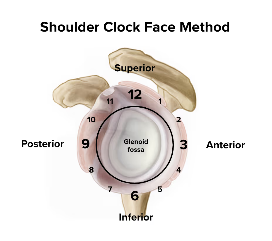
The clock face method solves this communication problem by using the glenoid (the socket of the shoulder) as a clock face when viewed from the side.
With this method:
12 o'clock is at the top (superior)
3 o'clock is to the right (anterior)
6 o'clock is at the bottom (inferior)
9 o'clock is to the left (posterior)
For example, instead of saying a labral tear is in the anterior-superior region, we can say it runs from 1 to 3 o'clock. Or if there's rotator cuff damage, we might say it's located at the 12 o'clock position.
This precision helps surgeons know exactly where to look and what to repair. The clock face method also guides our slice planning to ensure we capture anatomy at the correct angles.
How to Perform a Shoulder MRI with Clock Face Method
The step-by-step guide below will show you how to set up and perform a shoulder MRI protocol in practice.
We will perform the protocol in 3 parts:
Set up the Patient and MRI Scanner
Plan and Acquire the Protocol Sequences
Review the Images
Part 1: Set up the Patient and MRI Scanner
1. Position the Patient and Coils
Lay the patient head-first and supine (on their back) with the shoulder aligned at the scanner's isocenter.
Use a dedicated shoulder coil array or flexible coil that surrounds the entire shoulder region to ensure high-resolution imaging. This coil provides strong signal reception and full coverage of the joint, including the rotator cuff, labrum, and surrounding structures.
Once the patient is in place, review your scanner’s hardware settings.
In this guide, we will use the following settings:
Scanner Setting
Value
Why This Value
Magnetic field strength
1.5 T
Enables high Signal-to-Noise Ratio, which gives superior image quality.
Maximum gradient strength
45 mT/m
Enables faster acquisitions while preserving high image quality.
This hardware setup is widely used in clinical practice. It balances acquisition time, image quality, and patient comfort.
3. Capture the Initial Localizer Images
Before we can perform any MRI protocol, we must always capture initial localizer images of the patient. These images act as a guide for planning the detailed scans we will perform next.
We should always capture localizers in three planes:
Axial
Sagittal
Coronal
Once acquired, upload the initial localizer images into the three viewports.
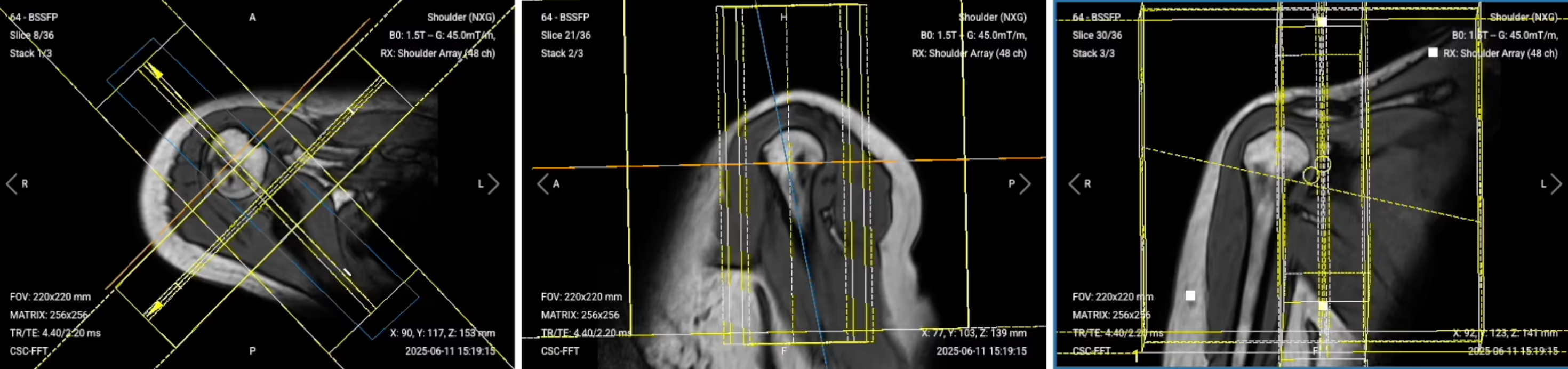
Then, scroll through each of the image stacks to locate a central slice that clearly shows the anatomy of the shoulder.
✅ Correct Setup of Localizer Images for Shoulder MRI:
Part 2: Plan and Acquire the Protocol Sequences
When all preparations are ready, we can start planning and acquiring the protocol sequences.
Let's go through the pulse sequences a standard shoulder MRI protocol includes, why we perform them, and how to set them up.
Planning Additional Localizers for the Clock Face Method
Before we acquire our high-resolution sequences, we need additional localizers to plan our sequences according to specific anatomical structures using the clock face method.
We’ll run two different localizer sequences:
Two-Plane Localizer (Sagittal and Coronal Views):
Axial PD Fat-Saturated Localizer
1. Two-Plane Localizer (Sagittal and Coronal Views):
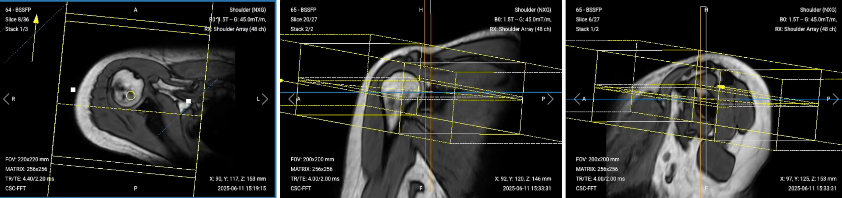
✅ Correct Planning:
Planning Instructions:
Use the glenoid fossa and rim as your anatomical references.
Align the slices as follows:
Sagittal localizer: Run parallel to the glenoid rim to visualize the glenohumeral joint clearly.
Coronal localizer: Run perpendicular to the glenoid rim, also showing the glenohumeral joint.
Both localizers share the same center and give us clear visualization of the glenoid fossa and rim.
Use appropriate geometry parameters:
Slice number: Enough to cover the shoulder region (12-15 slices).
Slice thickness: 5-6 mm for good overview imaging.
Slice gap: 1 mm to prevent crosstalk while maintaining coverage.
Set the fold-over direction (phase encoding) to anterior-posterior to reduce motion artifacts.
✅ Sagittal Localizer – Correct Image Example:
✅ Coronal Localizer – Correct Image Example:
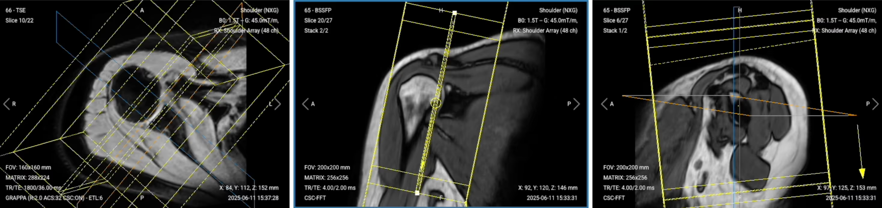
2. Axial PD Fat-Saturated Localizer:
✅ Correct Planning:
Planning Instructions:
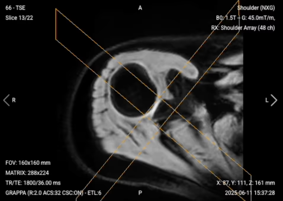
Use the supraspinatus tendon as your anatomical reference.
Align the slices as follows:
Sagittal localizer: Angle the slice package perpendicular to the glenoid bone tips.
Coronal localizer: Center slices over the glenohumeral joint.
Use appropriate geometry parameters:
Slice number: Enough to cover the shoulder joint and supraspinatus tendon area (20-25 slices).
Slice thickness: 4 mm for detailed visualization.
Slice gap: 0.8 mm to maintain anatomical continuity.
Set the fold-over direction (phase encoding) to anterior-posterior for straight shoulder view.
Center the field of view over the shoulder for optimal positioning.
The 6 Sequences of a Standard Shoulder MRI Protocol
Once we have all localizers, we will run the following 6 sequences:
Sagittal PD Fat-Saturated TSE
Coronal PD Fat-Saturated TSE
Axial PD Fat-Saturated TSE
Sagittal T1 TSE
Coronal T2 TSE
Axial T1 TSE
We mainly use Turbo Spin Echo sequences for this study. These sequences let us create multiple types of contrasts, including PD with fat suppression, T1, and T2 weighting. This helps us assess the integrity of the shoulder structures and check for common pathologies while maintaining high resolution for small structures.
The order of sequences is very important for the clock face method. Each sequence helps us plan the next one for optimal visualization of shoulder anatomy.
In the sections below, we go through how to plan and set up each sequence.
1. Sagittal PD Fat-Saturated TSE
✅ Correct Planning:
Planning Instructions:
Plan the stack using the sagittal and coronal localizers and axial localizer views.
Use the glenoid fossa and tips of the glenoid bone as your anatomical references.
Align the slices as follows:
Coronal localizer: Parallel to the upper and lower tips of the glenohumeral joint, connecting these two points.
Axial localizer: Parallel to the glenoid rim to follow the clock face orientation.
Sagittal localizer: Center the slice package properly for coverage from deltoid muscle to scapular notch.
Use appropriate geometry parameters:
Slice number: Enough to fully cover the shoulder region (29 slices).
Slice thickness: 3 mm for high resolution without sacrificing scan time or SNR.
Slice gap: 0.3 mm (10% of slice thickness) to enhance small structure visibility.
Set the fold-over direction (phase encoding) to anterior-posterior to reduce motion artifacts.
Parameters for Sagittal PD Fat-Saturated TSE:
Parameter
Recommended Values
Why These Values
Echo Time (TE)
20–40 ms
Shorter TE is required for PD contrast.
Repetition Time (TR)
1,500–2,500 ms
Longer TR is required for PD contrast.
Field-of-View (FOV)
160 × 160 mm
Small enough to focus on the shoulder region with high resolution.
Matrix
320 × 256
High matrix size to get excellent resolution for small shoulder structures while maintaining good SNR.
Foldover Direction (Phase)
Anterior-to-Posterior (AP)
To reduce motion artifacts and align with natural shoulder orientation.
Number of Slices
25–30
Enough slices to cover from deltoid muscle to scapular notch.
Slice Thickness
3 mm
Thin enough for high resolution without sacrificing scan time or SNR.
Slice Gap
0.3 mm
10% of slice thickness to enhance small structure visibility and maintain continuity.
NEX / Averages
1–2
To get enough SNR while keeping scan time reasonable.
Turbo Factor / ETL
6
Lower turbo factor to minimize T2-weighting and get purer PD contrast.
Bandwidth
100,000 Hz
High enough to avoid chemical shift artifacts without reducing SNR.
Fold-over Suppression
Yes
To avoid aliasing or wrap-around artifacts.
Fat Suppression
Spectral
To nullify fat signal and make soft tissues, tendons, and fluid-related abnormalities more visible.
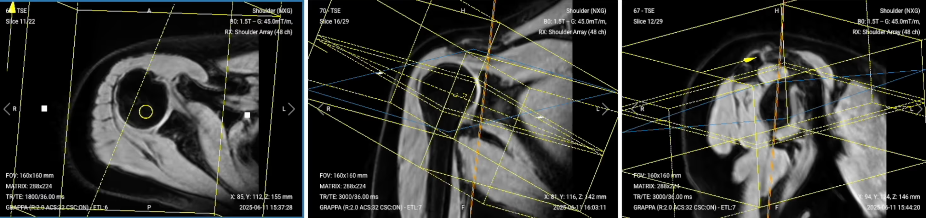
2. Coronal PD Fat-Saturated TSE
✅ Correct Planning:
Planning Instructions:
Plan the stack using the sagittal PD FS sequence we just acquired.
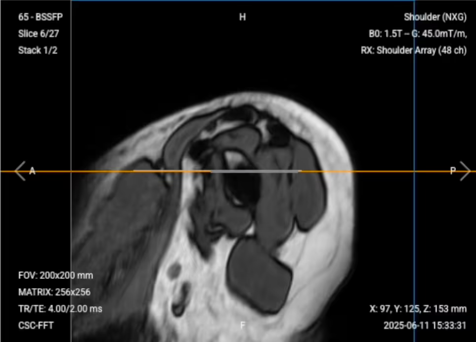
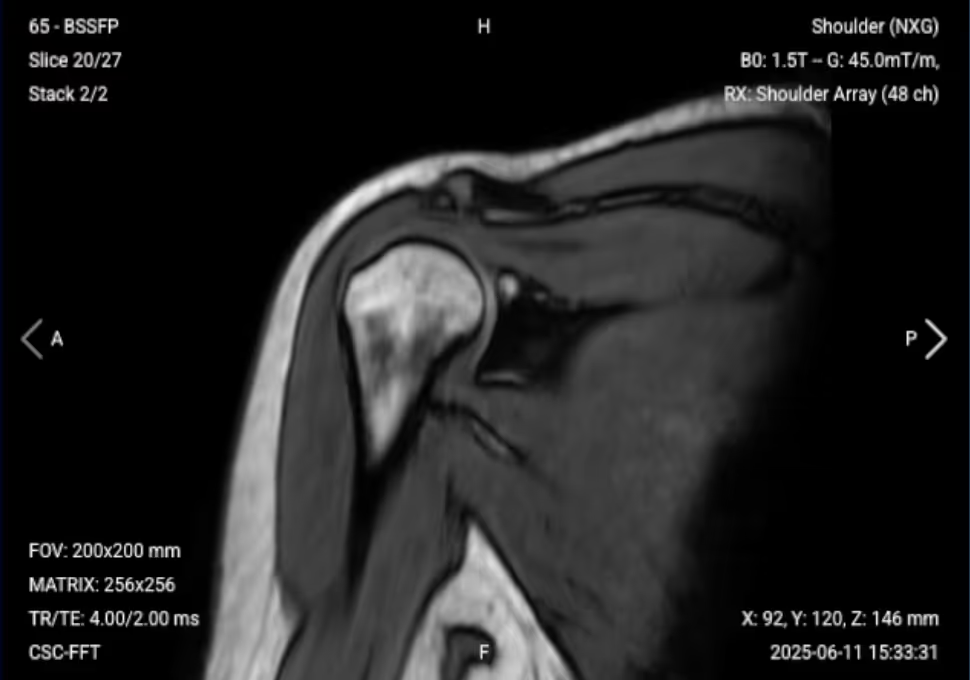
Use the glenoid fossa (12 o'clock to 6 o'clock positions) as your anatomical reference.
Align the slices as follows:
Sagittal PD FS: Orient from the 12 o'clock down to the 6 o'clock positions on the glenoid, connecting these two points using the clock face approach.
Axial localizer: You can align perpendicular to the glenoid rim for clear articular surface views, or parallel to the supraspinatus tendon for exceptional rotator cuff visualization (recommended).
Use appropriate geometry parameters:
Slice number: Enough to cover shoulder region from side to side.
Slice thickness: 3 mm for high resolution.
Slice gap: 0.3 mm to maintain small structure visibility.
Coverage should extend from the front portion of the coracoid process to two slices behind the humeral head.
Set the fold-over direction (phase encoding) to anterior-posterior for optimal image quality.
Parameters for Coronal PD Fat-Saturated TSE:
Parameter
Recommended Values
Why These Values
Echo Time (TE)
20–40 ms
Shorter TE is required for PD contrast.
Repetition Time (TR)
1,500–2,500 ms
Longer TR is required for PD contrast.
Field-of-View (FOV)
160 × 160 mm
Small enough to focus on the shoulder region with high resolution.
Matrix
320 × 256
High matrix size to get excellent resolution for small shoulder structures while maintaining good SNR.
Foldover Direction (Phase)
Anterior-to-Posterior (AP)
To reduce motion artifacts and align with natural shoulder orientation.
Number of Slices
25–30
Enough slices to cover from coracoid process to behind humeral head.
Slice Thickness
3 mm
Thin enough for high resolution without sacrificing scan time or SNR.
Slice Gap
0.3 mm
10% of slice thickness to enhance small structure visibility and maintain continuity.
NEX / Averages
1–2
To get enough SNR while keeping scan time reasonable.
Turbo Factor / ETL
6
Lower turbo factor to minimize T2-weighting and get purer PD contrast.
Bandwidth
100,000 Hz
High enough to avoid chemical shift artifacts without reducing SNR.
Fold-over Suppression
Yes
To avoid aliasing or wrap-around artifacts.
Fat Suppression
Spectral
To nullify fat signal and make soft tissues, tendons, and fluid-related abnormalities more visible.
3. Axial PD Fat-Saturated TSE
✅ Correct Planning:
Planning Instructions:
Plan the stack using the coronal PD FS sequence we just acquired.
Use the glenoid rim and clock face reference as your anatomical references.
Align the slices as follows:
Coronal sequence: Set perpendicular slice position on top of the coronal plane.
Sagittal sequence: Refer to the glenoid fossa as the face of the clock. Orient the angulation to the 9 to 3 o'clock position (drawing a line from left to right across the glenoid).
Use appropriate geometry parameters:
Slice number: Enough to cover from acromioclavicular joint to two slices below articular capsule.
Slice thickness: 3 mm for high resolution.
Slice gap: 0.3 mm to maintain anatomical continuity.
Position the field of view on the axial plane for a straight view (slices may appear skewed on other planes due to oblique shoulder angles).
Set the fold-over direction (phase encoding) to anterior-posterior for optimal imaging.
Parameters for Axial PD Fat-Saturated TSE:
Parameter
Recommended Values
Why These Values
Echo Time (TE)
20–40 ms
Shorter TE is required for PD contrast.
Repetition Time (TR)
1,500–2,500 ms
Longer TR is required for PD contrast.
Field-of-View (FOV)
160 × 160 mm
Small enough to focus on the shoulder region with high resolution.
Matrix
320 × 256
High matrix size to get excellent resolution for small shoulder structures while maintaining good SNR.
Foldover Direction (Phase)
Anterior-to-Posterior (AP)
To reduce motion artifacts and align with natural shoulder orientation.
Number of Slices
25–30
Enough slices to cover from acromioclavicular joint to below articular capsule.
Slice Thickness
3 mm
Thin enough for high resolution without sacrificing scan time or SNR.
Slice Gap
0.3 mm
10% of slice thickness to enhance small structure visibility and maintain continuity.
NEX / Averages
1–2
To get enough SNR while keeping scan time reasonable.
Turbo Factor / ETL
6
Lower turbo factor to minimize T2-weighting and get purer PD contrast.
Bandwidth
100,000 Hz
High enough to avoid chemical shift artifacts without reducing SNR.
Fold-over Suppression
Yes
To avoid aliasing or wrap-around artifacts.
Fat Suppression
Spectral
To nullify fat signal and make soft tissues, tendons, and fluid-related abnormalities more visible.
4. Sagittal T1 TSE
✅ Correct Planning:
Planning Instructions:
Copy the slice geometry and planning from the previous sagittal PD FS sequence.
Keep the same slice angulation, coverage, and positioning to ensure images of different contrasts can be clearly compared.
Parameters for Sagittal T1 TSE:
Parameter
Recommended Values
Why These Values
Echo Time (TE)
10 ms
Shorter TE is required for T1 contrast.
Repetition Time (TR)
400 ms
Shorter TR is required for T1 contrast.
Field-of-View (FOV)
160 × 160 mm
Small enough to focus on the shoulder region with high resolution.
Matrix
320 × 256
High matrix size to get excellent resolution for small shoulder structures while maintaining good SNR.
Foldover Direction (Phase)
Anterior-to-Posterior (AP)
To reduce motion artifacts and align with natural shoulder orientation.
Number of Slices
29
Enough slices to cover from deltoid muscle to scapular notch.
Slice Thickness
3 mm
Thin enough for high resolution without sacrificing scan time or SNR.
Slice Gap
0.3 mm
10% of slice thickness to enhance small structure visibility and maintain continuity.
NEX / Averages
1–2
To get enough SNR while keeping scan time reasonable.
Turbo Factor / ETL
2
Lower turbo factor for T1 contrast to minimize T2-weighting.
Bandwidth
100,000 Hz
High enough to avoid chemical shift artifacts without reducing SNR.
Fold-over Suppression
Yes
To avoid aliasing or wrap-around artifacts.
Fat Suppression
None
Not needed for T1 sequences.
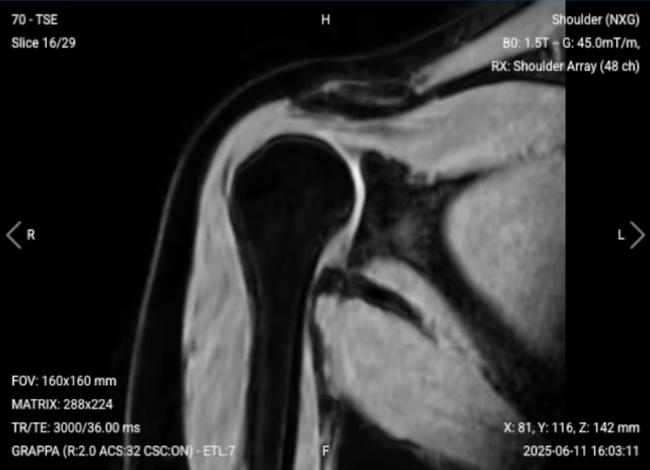
5. Coronal T2 TSE
✅ Correct Planning:
Planning Instructions:
Copy the slice geometry and planning from the previous coronal PD FS sequence.
Keep the same slice angulation, coverage, and positioning to ensure images of different contrasts can be clearly compared.
Parameters for Coronal T2 TSE:
Parameter
Recommended Values
Why These Values
Echo Time (TE)
30 ms
Moderate TE for T2 contrast while avoiding magic angle artifacts.
Repetition Time (TR)
3,000 ms
Longer TR is required for T2 contrast.
Field-of-View (FOV)
160 × 160 mm
Small enough to focus on the shoulder region with high resolution.
Matrix
320 × 256
High matrix size to get excellent resolution for small shoulder structures while maintaining good SNR.
Foldover Direction (Phase)
Anterior-to-Posterior (AP)
To reduce motion artifacts and align with natural shoulder orientation.
Number of Slices
25–30
Enough slices to cover from coracoid process to behind humeral head.
Slice Thickness
3 mm
Thin enough for high resolution without sacrificing scan time or SNR.
Slice Gap
0.3 mm
10% of slice thickness to enhance small structure visibility and maintain continuity.
NEX / Averages
1–2
To get enough SNR while keeping scan time reasonable.
Turbo Factor / ETL
12
Higher turbo factor to enhance T2 contrast and optimize scan time.
Bandwidth
100,000 Hz
High enough to avoid chemical shift artifacts without reducing SNR.
Fold-over Suppression
Yes
To avoid aliasing or wrap-around artifacts.
Fat Suppression
None
Not typically used for T2 sequences in shoulder imaging.
6. Axial T1 TSE
✅ Correct Planning:
Planning Instructions:
Copy the slice geometry and planning from the previous axial PD FS sequence.
Keep the same slice angulation, coverage, and positioning to ensure images of different contrasts can be clearly compared.
Parameters for Axial T1 TSE:
Parameter
Recommended Values
Why These Values
Echo Time (TE)
10 ms
Shorter TE is required for T1 contrast.
Repetition Time (TR)
400 ms
Shorter TR is required for T1 contrast.
Field-of-View (FOV)
160 × 160 mm
Small enough to focus on the shoulder region with high resolution.
Matrix
320 × 256
High matrix size to get excellent resolution for small shoulder structures while maintaining good SNR.
Foldover Direction (Phase)
Anterior-to-Posterior (AP)
To reduce motion artifacts and align with natural shoulder orientation.
Number of Slices
25–30
Enough slices to cover from acromioclavicular joint to below articular capsule.
Slice Thickness
3 mm
Thin enough for high resolution without sacrificing scan time or SNR.
Slice Gap
0.3 mm
10% of slice thickness to enhance small structure visibility and maintain continuity.
NEX / Averages
1–2
To get enough SNR while keeping scan time reasonable.
Turbo Factor / ETL
2
Lower turbo factor for T1 contrast to minimize T2-weighting.
Bandwidth
100,000 Hz
High enough to avoid chemical shift artifacts without reducing SNR.
Fold-over Suppression
Yes
To avoid aliasing or wrap-around artifacts.
Fat Suppression
None
Not needed for T1 sequences.
How to Avoid Artifacts When Planning the Sequences
The table below lists the 5 common shoulder artifacts, and what techniques you can use to avoid them:
Artifacts
Solution – How to Avoid It
Motion artifacts
Shorten the scan time to reduce the risk of patient movement.
Magic angle artifacts
Acquire T2-weighted images to check if the signal is artifact or real tendon pathology.
Chemical shift artifacts
Increase the bandwidth to reduce spatial shift between fat and water signals.
Wrap-around artifacts
Activate fold-over suppression to block signals from anatomy outside the field of view.
Susceptibility artifacts
Use spin echo sequences instead of gradient echo sequences.
Cross-talk artifacts
Keep enough slice gap to prevent overlap between slices.
Part 3: Review the Images
Finally, we will review the images to ensure all the anatomical information we need is clear.
These key structures must be clearly visible in a shoulder MRI:
Below, we will go through all the different image contrasts and explain their specific role in imaging the shoulder.
PD Fat-Saturated – Best for Soft Tissue, Labral, and Rotator Cuff Pathology
Proton Density Fat-Saturated (PD FS) imaging provides excellent soft tissue contrast while suppressing fat, making it ideal for evaluating shoulder joint structures.
In shoulder MRI, PD FS sequences are the gold standard for detecting rotator cuff tears, labral injuries, and joint effusions. They enhance soft tissues and fluids without fat signal interference, making tears appear as bright signal that interrupts the normally dark tendon or labrum. This contrast is optimal for detecting subtle tendinosis and capsular pathologies.
The three planes captured in PD FS provide comprehensive coverage. Each plane helps plan the next using the clock face method, ensuring optimal visualization of all shoulder structures.
✅ Sagittal PD FS of the Shoulder – Correct Image Example:
Things to Look for in Sagittal PD FS:
Glenoid fossa clearly outlined with good contrast
Coracoid process visible and well-defined
Supraspinatus tendon integrity along its full length
Joint effusion or fluid collections appearing bright
✅ Coronal PD FS of the Shoulder – Correct Image Example:
Things to Look for in Coronal PD FS:
Supraspinatus tendon displayed throughout its length in single slices
Clear visualization of rotator cuff insertions
Labral morphology and signal intensity
Acromioclavicular joint and subacromial space
✅ Axial PD FS of the Shoulder – Correct Image Example:
Things to Look for in Axial PD FS:
Labrum appearing as a small dark structure around the glenoid
Rotator cuff tendons (infraspinatus, subscapularis, superior glenohumeral ligament)
Complete coverage from the acromioclavicular joint downward
Biceps tendon and bicipital groove pathology
T1 TSE – Highlight Fat-Containing Tissues and Anatomical Structure
T1-weighted imaging makes fat appear bright and fluid dark. This contrast is ideal for fat-rich tissues and structural abnormalities. T1 shows anatomical structures clearly since it helps us see where different solid tissues like muscle and fat meet.
In shoulder MRI, T1 sequences are valuable for evaluating bone marrow pathology, fatty infiltration of muscles, and overall anatomical structure. T1 contrast helps identify bone marrow changes, muscle atrophy, and provides baseline anatomy for comparison with other sequences
✅ Sagittal T1 of the Shoulder – Correct Image Example:
Things to Look for in Sagittal T1:
Bone marrow signal intensity and any pathological changes
Muscle anatomy and fatty infiltration patterns
Structural integrity compared to PD FS sequences
Overall glenohumeral joint alignment
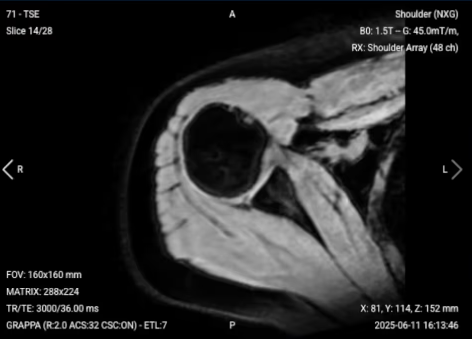
✅ Axial T1 of the Shoulder – Correct Image Example:
Things to Look for in Axial T1:
Fatty infiltration of rotator cuff muscles
Bone marrow changes in the humeral head or glenoid
Muscle volume and atrophy assessment
Comparison with PD FS for structure evaluation
T2 TSE – Highlight Fluid-Related Tissues and Inflammation
T2-weighted imaging makes fluids appear bright. This contrast is ideal for detecting tissues and abnormalities with high water content.
In shoulder MRI, T2 sequences help confirm pathology seen on other sequences and distinguish real inflammation from magic angle artifacts. They are particularly useful for evaluating edema, inflammation, joint effusions, and confirming whether increased signal on other sequences represents true pathology.
✅ Coronal T2 of the Shoulder – Correct Image Example:
Things to Look for in Coronal T2:
Joint effusion and synovial thickening
Bone marrow edema appearing bright
Confirmation of tendon pathology versus magic angle artifact
Fluid collections in the subacromial-subdeltoid bursa
Final Checks:
Before finishing a shoulder MRI, always check these 5 points to ensure diagnostic quality:
Rotator Cuff Coverage: All four rotator cuff tendons must be clearly visible with sharp definition, especially the supraspinatus throughout its length in coronal PD FS.
Labral Visualization: The glenoid labrum must appear as a dark triangular structure around the glenoid in axial and coronal views with high resolution.
Clock Face Alignment: Slices must be properly angled according to glenoid anatomy, with coronal views following 12-6 o'clock and axial views following 9-3 o'clock orientation.
Fat Suppression Quality: PD FS sequences must show uniform fat suppression so that soft tissue abnormalities and fluid appear clearly without fat signal interference.
Image Quality and Coverage: All sequences must have strong SNR, excellent spatial resolution for small structures, and complete coverage from acromioclavicular joint to inferior glenohumeral joint.

.svg)