This step-by-step guide is for MRI students, radiographers and technologists who wish to improve their planning skills and master the routine brain MRI protocol.
What you will learn:
Key factors in brain MRIs, including trade-offs.
Patient and scanner setup tips.
Best pulse sequences and planning techniques.
Ways to avoid common artifacts.
What great brain images should look like.
Key Takeaways
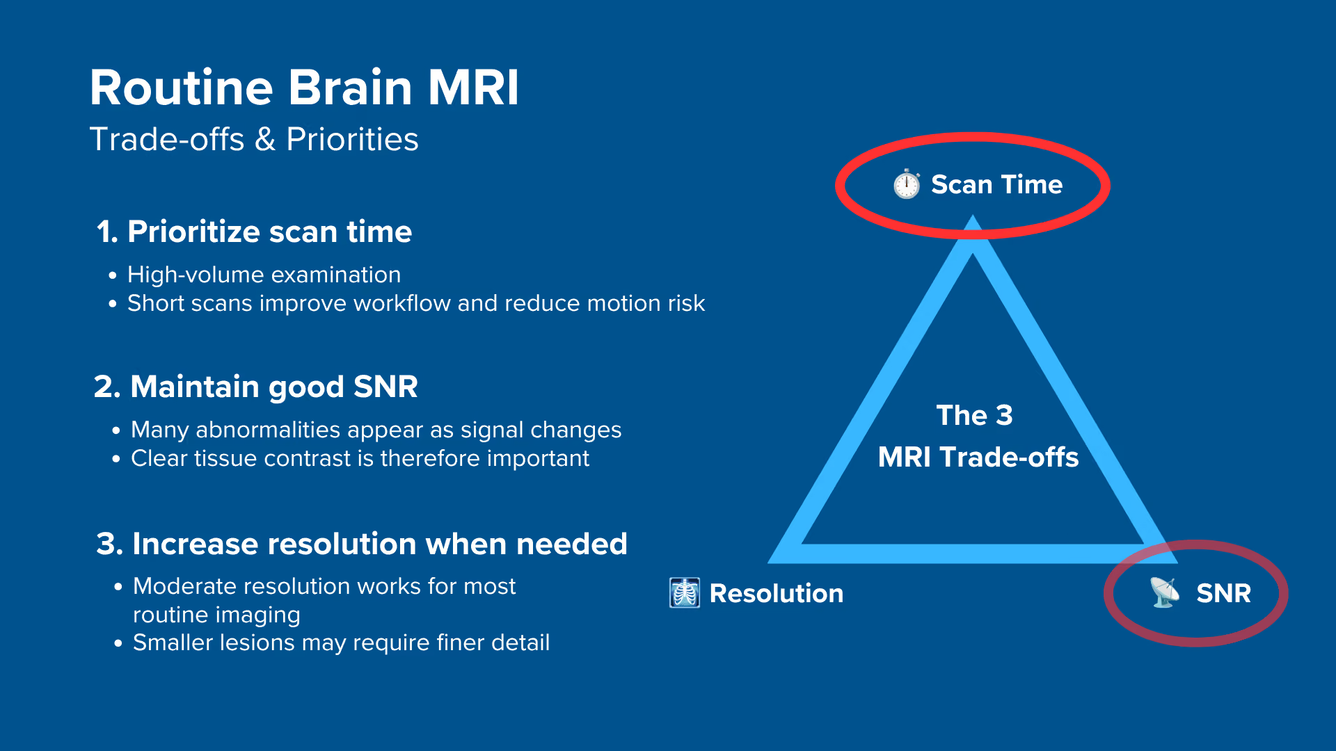
For routine brain MRIs, it's generally recommended to prioritize scan time, followed by SNR and resolution.
A routine brain MRI is one of the most requested protocols, so a short scan time usually comes first. Most brain pathologies are identified by signal differences, so strong SNR generally matters more than fine detail. For smaller lesions, higher resolution is needed.
We mainly use Fast/Turbo Spin Echo sequences in routine brain MRIs.
These sequences give fast, high-quality images with strong contrast and relatively few artifacts, which makes them well-suited to routine clinical imaging. They let us produce T1 and T2 contrast, and add an inversion pulse that nulls the CSF signal for FLAIR. Together, these help us assess brain structure and detect abnormalities.
Avoid these 6 common brain artifacts.
Artifacts
Solution: How to Avoid It
Motion artifacts
Shorten the scan time to reduce the risk of patient movement.
Susceptibility artifacts
Spin echo loses less signal to field inhomogeneity than gradient echo. The DWI readout still distorts, so keep its bandwidth high and its slices away from the sinuses.
Chemical shift artifacts
Increase the bandwidth to reduce the spatial displacement between fat and water signals.
CSF flow artifacts
FLAIR reduces this by nulling CSF that received a clean inversion, though 2D FLAIR can still show inflow artifact near the ventricles. Where it persists, add flow compensation gradients.
Truncation artifacts
Ringing at sharp boundaries comes from sampling a finite region of k-space, so raise the phase matrix rather than the field of view. It is reduced rather than removed.
Wrap-around artifacts
Extend the phase field of view beyond the anatomy so nothing outside it can fold in. Activate fold-over suppression only if the field of view cannot be extended.
Intro to Brain MRIs
The brain is a complex organ responsible for controlling all body functions, processing sensory information, and enabling cognitive abilities. Because of its importance and the range of pathologies that affect it, the brain is one of the most frequently examined areas in MRI.
Brain MRI protocols are used to diagnose a wide range of neurological conditions, including tumors, strokes and multiple sclerosis, as well as psychiatric disorders that affect brain function.
How to Balance the 3 Trade-offs in Routine Brain MRIs
In MRI, we always face a trade-off between 3 key metrics. Contrast and slice thickness are tied into the same balance, so changing any one of these affects the others:
Scan Time: How fast a pulse sequence can be completed.
Resolution: How much detail the image can display.
SNR: How clear the image is, how much signal relative to noise.
Improving one of these metrics reduces the performance of the others. To decide what trade-offs to make, we must consider the needs of each clinical situation.
For routine brain MRIs, it’s generally true that:
It’s one of the most highly requested protocols, so a short scan time is usually the priority.
Most brain pathologies are identified primarily by signal differences rather than fine structural details.
When checking for smaller lesions, a higher resolution is needed.
Therefore, we typically:
Prioritize scan time, since routine brain MRI is performed frequently and the protocol needs to remain practical for a busy clinical list.
Maintain good SNR so that differences in tissue signal remain clear, particularly on sequences where lesion detection depends strongly on contrast.
Increase resolution when needed for smaller or more subtle lesions, rather than maximizing spatial detail across every routine sequence.
Note! Prioritizing scan time in brain MRIs is only a general guideline, NOT a strict rule. If you need to visualize finer details or if short scan time is less urgent, your priorities may shift. The right balance always depends on the needs of your patient and clinic.
One more lever sits outside these three. Parallel imaging, offered as SENSE or GRAPPA, skips phase-encoding steps and reconstructs the missing data from coil sensitivity information. It buys back scan time at a modest SNR cost, which is what makes thinner slices and fuller coverage affordable in a protocol where scan time is the first priority.
Brain Health Conditions and the MRI Sequences That Reveal Them
The brain MRI study can help us diagnose a wide range of health conditions. The table below lists some of the most common conditions, and what pulse sequences that reveal them:
Common Brain Conditions
Clearly Seen on Sequence
Why This Sequence?
Anatomical structures and lesions:
• Tumors
• Subacute hemorrhage
• Metastases
• Bone marrow changes
T1 TSE
Provides clear gray-white differentiation and baseline for contrast assessment. Detects T1 hyperintense findings like subacute hemorrhage and marrow pathology. Contrast-enhanced T1 improves tumor and metastasis visibility.
Highlights water-rich tissues, making it ideal for detecting edema, inflammation, and CSF-related abnormalities. Helps assess fluid accumulation and tissue changes.
White matter and ischemic lesions:
• Multiple sclerosis (MS)
• Small vessel disease
• Chronic ischemia
• Gliosis
T2 FLAIR
Suppresses CSF signal while preserving sensitivity to pathological water, making white matter lesions highly visible. Ideal for detecting demyelination, chronic ischemia, and gliosis, especially near ventricles where bright CSF on T2 could obscure lesions.
Detects restricted water molecule movement in acute ischemic tissue within minutes of onset, long before other sequences. It’s the core sequence for rapid stroke treatment decisions.
How to Perform a Routine Brain MRI
The step-by-step guide below will show you how to set up and perform a routine brain MRI protocol in practice.
We will perform the protocol in 3 parts:
Set up the Patient and MRI Scanner
Plan and Acquire the Protocol Sequences
Review the Images
Part 1: Set up the Patient and MRI Scanner
1. Position the Patient in the Scanner
Lay the patient head-first and supine (on their back) with the head centered at the scanner's isocenter.
Use a dedicated head coil. It gives strong signal reception across the whole brain, which leaves enough SNR for high in-plane resolution. In the Corsmed simulator this is Head Birdcage Rx. The video uses Optimal Rx, which gives the best signal available in the simulation.
Once the patient is in place, review your scanner’s hardware settings.
In this guide, we will use the following settings:
Scanner Setting
Value
Why This Value
Magnetic field strength
1.5 T
The most common clinical field strength, giving enough SNR for this protocol with less susceptibility and B1 artifact than 3 T.
Maximum gradient strength
45 mT/m
Provides strong, versatile gradient performance that supports fast imaging and precise spatial encoding.
This hardware setup is widely used in clinical practice. It balances acquisition time, image quality, and patient comfort.
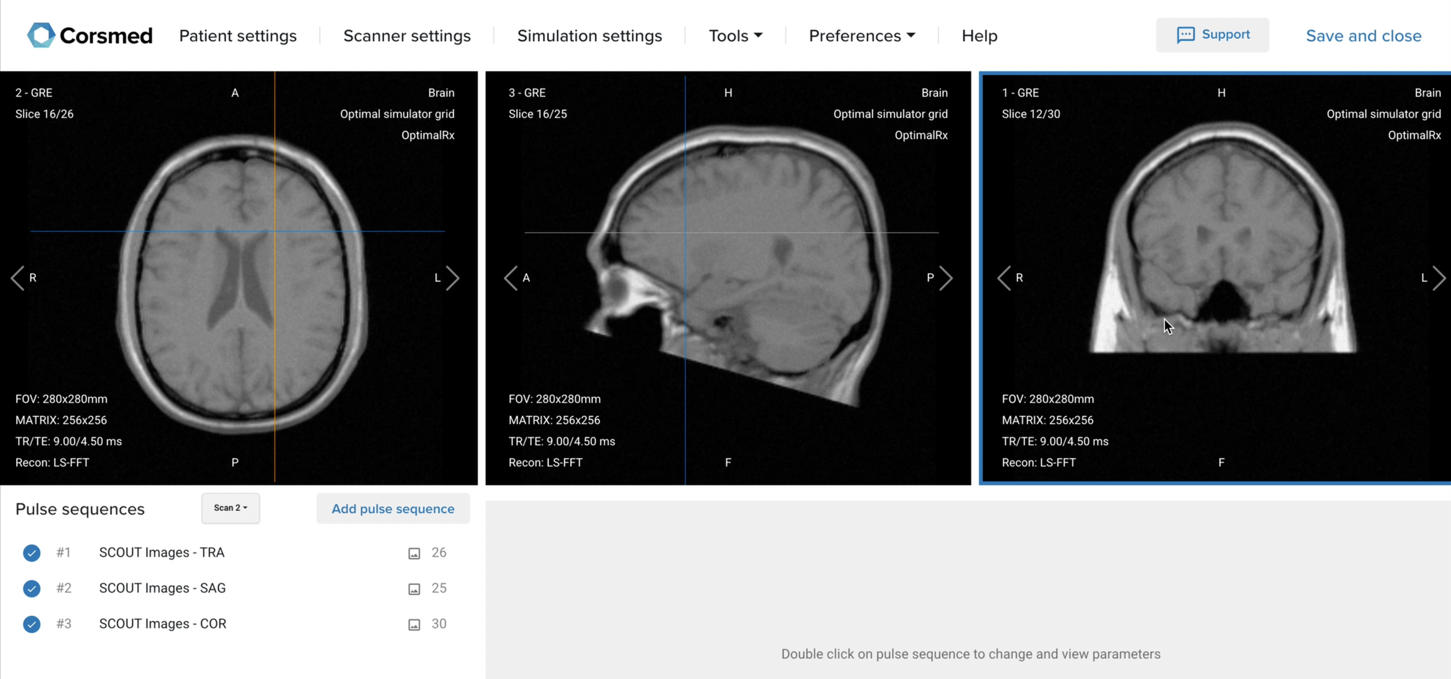
3. Capture the Initial Localizer Images
Before we can perform any MRI protocol, we must always capture initial localizer images of the patient. These images act as a guide for planning the detailed scans we will perform next.
We should always capture localizers in three planes:
Axial
Sagittal
Coronal
Once acquired, load the initial localizer images into the three viewports.
Then, scroll through each of the image stacks to locate a central slice that clearly shows the anatomy of the brain.
✅ Correct Setup of Localizer Images for Routine Brain MRI:
Part 2: Plan and Acquire the Protocol Sequences
When all preparations are ready, we can start planning and acquiring the protocol sequences.
Let’s go through the pulse sequences that a standard brain MRI protocol includes, why we perform them, and how to set them up.
The 6 Sequences of a Standard Brain MRI Protocol
Axial T2 TSE
Axial T2 FLAIR
Axial T1 TSE
Sagittal T1 TSE
Coronal T1 TSE
Diffusion-Weighted Imaging (DWI)
These six sequences make up the routine brain study. If the referral raises a question about blood, calcification or microhemorrhage, a susceptibility-sensitive sequence is added, either a T2*-weighted gradient echo or SWI, because those findings are detected there rather than on any of the six sequences below.
We mainly use fast or turbo spin echo sequences for this study. These sequences give fast, high-quality images with strong contrast and relatively few artifacts, which makes them well suited to routine clinical imaging.
Turbo spin echo sequences also let us create several types of contrast, including T2, T1, and inversion recovery contrast, which is what allows FLAIR to null the signal from cerebrospinal fluid.
This helps us assess the brain's structure, detect abnormalities, and identify common pathologies like tumors, strokes, and demyelination.
In the sections below, we go through how to plan and set up each sequence.
1. Axial T2 TSE
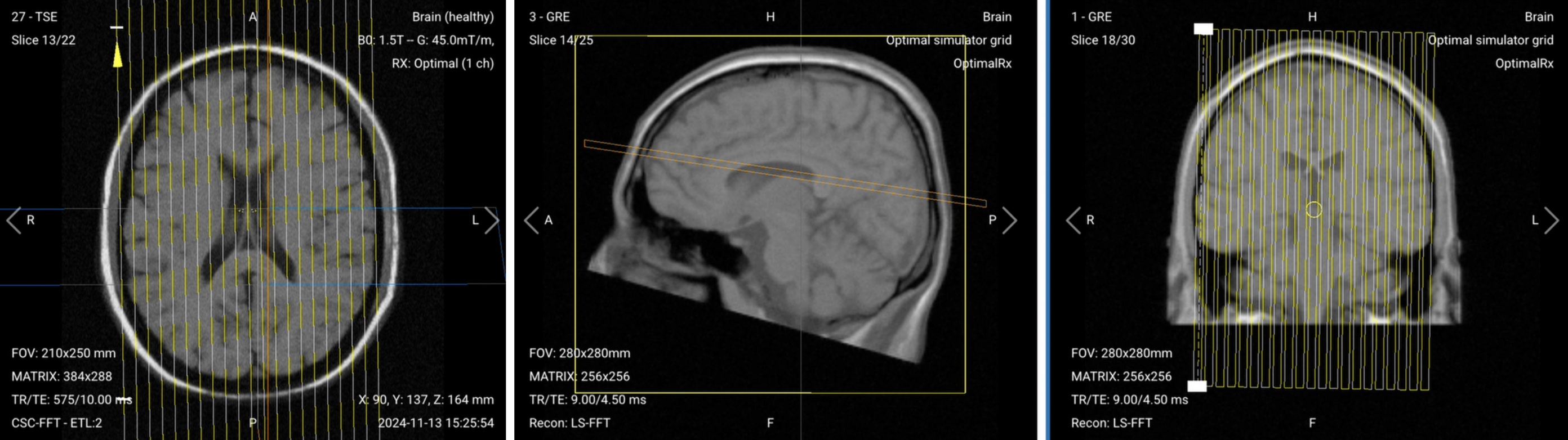
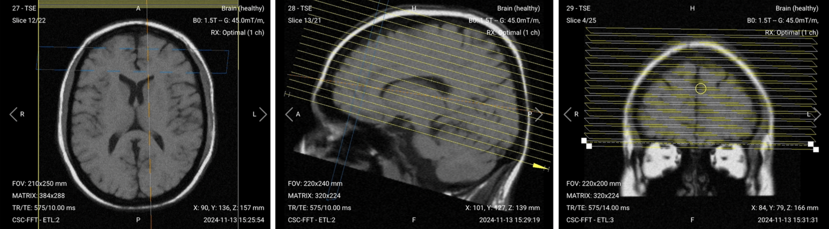
✅ Correct Planning:
Planning Instructions:
Use the corpus callosum as the anatomical reference.
Align the slices as follows:
Sagittal Localizer: Parallel to the anterior commissure-posterior commissure (AC-PC) line. This can also be aligned using the genu (front) and splenium (back) of the corpus callosum.
Coronal Localizer: Perpendicular to the mid-sagittal line, which runs from the superior sagittal sinus through the third ventricle to the base of the skull.
Add enough slices to cover from the vertex (top of the head) to the base of the skull.
Center the slices, then set the slice thickness and gap to the values in the table below.
Extend the field of view in the phase direction beyond the anatomy, so the nose does not wrap into the brain. This is not the same control as fold-over suppression, which several clinical scanners implement as extra phase data that is acquired and then discarded, under names like phase oversampling or no phase wrap. Extending the field of view is the better choice here, because the extra coverage is anatomy worth keeping.
Parameters for Axial T2 TSE:
Parameter
Recommended Values
Why These Values
Echo Time (TE)
100–130 ms
Long TE is required for T2 contrast.
Repetition Time (TR)
4,000–6,000 ms
Long TR is required for T2 contrast.
Field of View (FOV)
210 x 250 mm
Large enough to cover and fit the shape of the brain while avoiding wrap-around artifacts.
Matrix
384 x 288
~0.55 × 0.87 mm in-plane, fine enough for cortical and periventricular detail.
Foldover Direction (Phase)
Anterior-to-Posterior (AP)
Aligned with the extended phase FOV; keeps any residual ghosting along AP.
Number of Slices
24–26
Covers the whole brain from vertex to the base of the skull.
Slice Thickness
5 mm
At or below the 5 mm ceiling recommended for brain imaging, while keeping enough signal per slice to avoid extra averages.
Slice Gap
1 mm
20% of slice thickness, which limits cross-talk without hiding anatomy.
NEX / Averages
1–2
To get enough SNR, while keeping scan time short.
Turbo Factor / ETL
16–24
Higher turbo factor reduces scan time, and long effective TE provides T2 weighting.
Bandwidth per pixel
250–320 Hz/px
Moderate bandwidth balances chemical shift against SNR.
Fold-over Suppression
No
Not needed. The extended phase FOV already prevents wrap-around.
2. Axial T2 FLAIR
✅ Correct Planning:
Planning Instructions:
Copy the slice geometry and planning from the axial T2 sequence.
Keep the same slice angulation, coverage, and positioning to ensure images of different contrasts can be clearly compared.
Parameters for Axial T2 FLAIR:
Parameter
Recommended Values
Why These Values
Echo Time (TE)
100–140 ms
Produces T2 contrast under the inversion pulse.
Repetition Time (TR)
8,000–10,000 ms
Lets CSF magnetization recover fully before the next inversion pulse, so the null holds.
Inversion Time (TI)
2,200–2,500 ms
Matched to the point where CSF magnetisation crosses zero, which is what nulls its signal. The null shifts with TR, so a TI that works at one TR will not work at another.
Field of View (FOV)
210 x 250 mm
Large enough to cover and fit the shape of the brain while avoiding wrap-around artifacts.
Matrix
384 x 288
~0.55 × 0.87 mm in-plane, fine enough for cortical and periventricular detail.
Foldover Direction (Phase)
Anterior-to-Posterior (AP)
Aligned with the extended phase FOV; keeps any residual ghosting along AP.
Number of Slices
24–26
Covers the whole brain from vertex to the base of the skull.
Slice Thickness
5 mm
At or below the 5 mm ceiling recommended for brain imaging, while keeping enough signal per slice to avoid extra averages.
Slice Gap
1 mm
20% of slice thickness, which limits cross-talk without hiding anatomy.
NEX / Averages
1–2
To get enough SNR, while keeping scan time short.
Turbo Factor / ETL
16–24
Higher turbo factor reduces scan time, and long effective TE provides T2 weighting.
Bandwidth per pixel
250–320 Hz/px
Moderate bandwidth balances chemical shift against SNR.
Fold-over Suppression
No
Not needed. The extended phase FOV already prevents wrap-around.
Fat Suppression
None by default
Add Spectral only when orbital or scalp fat is obscuring the target, since suppression is unreliable near the sinuses and skull base.
A note on averages in FLAIR:
FLAIR is the noisiest sequence in this protocol, because nulling the CSF signal also removes signal that would otherwise contribute to the image. Acquiring it with a single average keeps the scan short, but the result can be noticeably grainy, and fine structures such as the layers around the suppressed CSF spaces become hard to separate.
Going from one average to two doubles the acquisition time and improves SNR by roughly 40%. Which choice is right depends on the question being asked. If the noise level still answers the referral, one average is the better use of the slot. If subtle periventricular lesions are the point of the study, two averages is worth the extra time.
3. Axial T1 TSE
✅ Correct Planning:
Planning Instructions:
Copy the slice geometry and planning from the axial T2 sequence.
Keep the same slice angulation, coverage, and positioning to ensure images of different contrasts can be clearly compared.
Parameters for Axial T1 TSE:
Parameter
Recommended Values
Why These Values
Echo Time (TE)
10–20 ms
Short TE is required for T1 contrast.
Repetition Time (TR)
400–600 ms
Short TR is required for T1 contrast.
Field of View (FOV)
210 x 250 mm
Large enough to cover and fit the shape of the brain while avoiding wrap-around artifacts.
Matrix
384 x 288
~0.55 × 0.87 mm in-plane, fine enough for cortical and periventricular detail.
Foldover Direction (Phase)
Anterior-to-Posterior (AP)
Aligned with the extended phase FOV; keeps any residual ghosting along AP.
Number of Slices
24–26
Covers the whole brain from vertex to the base of the skull.
Slice Thickness
5 mm
At or below the 5 mm ceiling recommended for brain imaging, while keeping enough signal per slice to avoid extra averages.
Slice Gap
1 mm
20% of slice thickness, which limits cross-talk without hiding anatomy.
NEX / Averages
1–2
To get enough SNR, while keeping scan time short.
Turbo Factor / ETL
2–4
Kept short so the effective TE stays short, preserving T1-weighting.
Bandwidth per pixel
250–320 Hz/px
Moderate bandwidth balances chemical shift against SNR.
Fold-over Suppression
No
Not needed. The extended phase FOV already prevents wrap-around.
4. Sagittal T1 TSE
✅ Correct Planning:
Planning Instructions:
Use the mid-sagittal line as the anatomical reference.
Align the slices as follows:
Coronal Localizer: Lay the slice package onto the mid-sagittal line, which runs from the superior sagittal sinus, through the third ventricle, down to the base of the skull.
Axial Localizer: Check that the package stays parallel to that same line, so the slices are not rotated relative to the head.
Add enough slices to cover the brain from side to side.
Set the fold-over direction to anterior-posterior.
Parameters for Sagittal T1 TSE:
Parameter
Recommended Values
Why These Values
Echo Time (TE)
10–20 ms
Short TE is required for T1 contrast.
Repetition Time (TR)
400–600 ms
Short TR is required for T1 contrast.
Field of View (FOV)
220 x 240 mm
Large enough to cover the brain while avoiding wrap-around artifacts.
Matrix
320 x 224
~0.69 × 1.07 mm in-plane. Coarser than the axials since this series is for midline orientation, not lesion detection.
Foldover Direction (Phase)
Anterior-to-Posterior (AP)
Keeps neck and shoulder signal from folding into the brain.
Number of Slices
24–26
Enough slices to cover the brain from side to side, ear to ear.
Slice Thickness
5 mm
At or below the 5 mm ceiling recommended for brain imaging, while keeping enough signal per slice to avoid extra averages.
Slice Gap
1 mm
20% of slice thickness, which limits cross-talk without hiding anatomy.
NEX / Averages
1–2
To get enough SNR, while keeping scan time short.
Turbo Factor / ETL
2–4
Kept short so the effective TE stays short, preserving T1-weighting.
Bandwidth per pixel
250–320 Hz/px
Moderate bandwidth balances chemical shift against SNR.
Fold-over Suppression
No
The 240 mm phase FOV covers the head front to back, and neck signal falls along the readout axis where it cannot fold in.
5. Coronal T1 TSE
✅ Correct Planning:
Planning Instructions:
Use the mid-sagittal line and AC-PC line as anatomical references.
Align the slices as follows:
Axial Localizer: Position slices perpendicular to the mid-sagittal line.
Sagittal Localizer: Position slices perpendicular to the AC-PC line.
Add enough slices to cover the brain from anterior to posterior.
Set the fold-over direction to right-left.
Parameters for Coronal T1 TSE:
Parameter
Recommended Values
Why These Values
Echo Time (TE)
10–20 ms
Short TE is required for T1 contrast.
Repetition Time (TR)
400–600 ms
Short TR is required for T1 contrast.
Field of View (FOV)
220 x 200 mm
Large enough to cover the brain while avoiding wrap-around artifacts.
Matrix
320 x 224
~0.69 × 0.89 mm in-plane, enough for temporal lobe and hippocampal detail.
Foldover Direction (Phase)
Right-to-Left (RL)
The head is narrower left to right than head to foot in this plane, so RL needs fewer phase steps and keeps the scan short.
Number of Slices
28–30
The brain is deeper front to back than it is tall, so the coronal package needs more slices.
Slice Thickness
5 mm
At or below the 5 mm ceiling recommended for brain imaging, while keeping enough signal per slice to avoid extra averages.
Slice Gap
1 mm
20% of slice thickness, which limits cross-talk without hiding anatomy.
NEX / Averages
1–2
To get enough SNR, while keeping scan time short.
Turbo Factor / ETL
2–4
Kept short so the effective TE stays short, preserving T1-weighting.
Bandwidth per pixel
250–320 Hz/px
Moderate bandwidth balances chemical shift against SNR.
Fold-over Suppression
No
The 200 mm phase FOV covers the full width of the head, so there is nothing outside it to fold in.
6. Axial Diffusion-Weighted Imaging (DWI)
✅ Correct Planning:
Planning Instructions:
Copy the slice geometry and planning from the axial sequences.
Adjust the slices as follows:
Sagittal Localizer: Shift the slice package superiorly so the paranasal sinuses and the mouth stay outside the slices. Air in these spaces has very different magnetic properties from brain tissue and causes susceptibility artifacts. If the anatomy still places the sinuses inside the package, angle it until they fall outside, while keeping the whole brain covered.
Coronal Localizer: Ensure the scan remains perpendicular to the mid-sagittal line.
Resolution on DWI is bounded from both directions. Going much above a 128 matrix lengthens the echo train, which adds distortion, costs SNR and blurs the image, so higher is not better here the way it is on a turbo spin echo. Going much below it pushes the pixel area past the 4 mm² limit used for stroke imaging and risks losing small infarcts to partial volume effects.
Parameters for Axial DWI:
Parameter
Recommended Values
Why These Values
Echo Time (TE)
70–100 ms
Set by the diffusion gradient pair, not chosen directly for contrast.
Repetition Time (TR)
4,000–6,000 ms
Removes T1 influence and fits all slices into one TR.
Field of View (FOV)
210 x 250 mm
Large enough to cover and fit the shape of the brain while avoiding wrap-around artifacts.
Matrix
128 x 128
~1.64 × 1.95 mm in-plane, a 3.2 mm² pixel area, which is the practical ceiling for single-shot EPI and fine enough to resolve a small infarct.
Foldover Direction (Phase)
Anterior-to-Posterior (AP)
To contain geometric distortions to the AP direction rather than the left-right axis, where distortion would be harder to read around.
Number of Slices
24–26
Matches the axial coverage, because an infarct at the vertex or in the posterior fossa must not fall outside the slices.
Slice Thickness
5 mm
At or below the 5 mm ceiling recommended for brain imaging, while keeping enough signal per slice to avoid extra averages.
Slice Gap
1 mm
20% of slice thickness, which limits cross-talk without hiding anatomy.
NEX / Averages
2–4
EPI at b=1000 is signal-starved, so averaging is needed here more than on the spin echo sequences.
Turbo Factor / ETL
N/A
This sequence uses a spin echo with an echo-planar readout, so there is no turbo train to set.
Bandwidth per pixel
600–800 Hz/px
Shortens EPI echo spacing, which limits distortion and lowers the minimum TE.
Fold-over Suppression
No
The 250 mm phase FOV already extends beyond the anatomy front to back.
B-value
0 and 1,000 s/mm²
The standard routine brain pair: b=0 is the unweighted reference and b=1000 gives strong sensitivity to restricted diffusion. Some protocols add 500 s/mm² for specialized assessments.
Scan mode
3-scan trace
Combines three gradient directions so no lesion is missed on an unmeasured axis.
b=0 Reference Image
Produced automatically
The unweighted reference that the ADC map is calculated against.
Output Trace DWI
Yes
Produces the trace image that acute infarcts appear bright on.
Output ADC
Yes
Produces the ADC map, which separates true restricted diffusion from T2 shine-through.
How to Avoid Artifacts When Planning the Sequences
The table below lists the 6 common brain artifacts, and what techniques you can use to avoid them:
Artifacts
Solution: How to Avoid It
Motion artifacts
Shorten the scan time to reduce the risk of patient movement.
Susceptibility artifacts
Spin echo loses less signal to field inhomogeneity than gradient echo. The DWI readout still distorts, so keep its bandwidth high and its slices away from the sinuses.
Chemical shift artifacts
Increase the bandwidth to reduce the spatial displacement between fat and water signals.
CSF flow artifacts
FLAIR reduces this by nulling CSF that received a clean inversion, though 2D FLAIR can still show inflow artifact near the ventricles. Where it persists, add flow compensation gradients.
Truncation artifacts
Ringing at sharp boundaries comes from sampling a finite region of k-space, so raise the phase matrix rather than the field of view. It is reduced rather than removed.
Wrap-around artifacts
Extend the phase field of view beyond the anatomy so nothing outside it can fold in. Activate fold-over suppression only if the field of view cannot be extended.
Part 3: Review the Images
Finally, we will review the images to ensure all the anatomical information we need is clear.
These key structures must be clearly visible in a brain MRI:
Gray and white matter
Ventricles and cerebrospinal fluid spaces
Basal ganglia
Brain stem and cerebellum
Corpus callosum
Major vessels at the skull base, seen as flow voids rather than as an angiographic assessment
Below, we will go through all the different image contrasts and explain their specific role in imaging the brain.
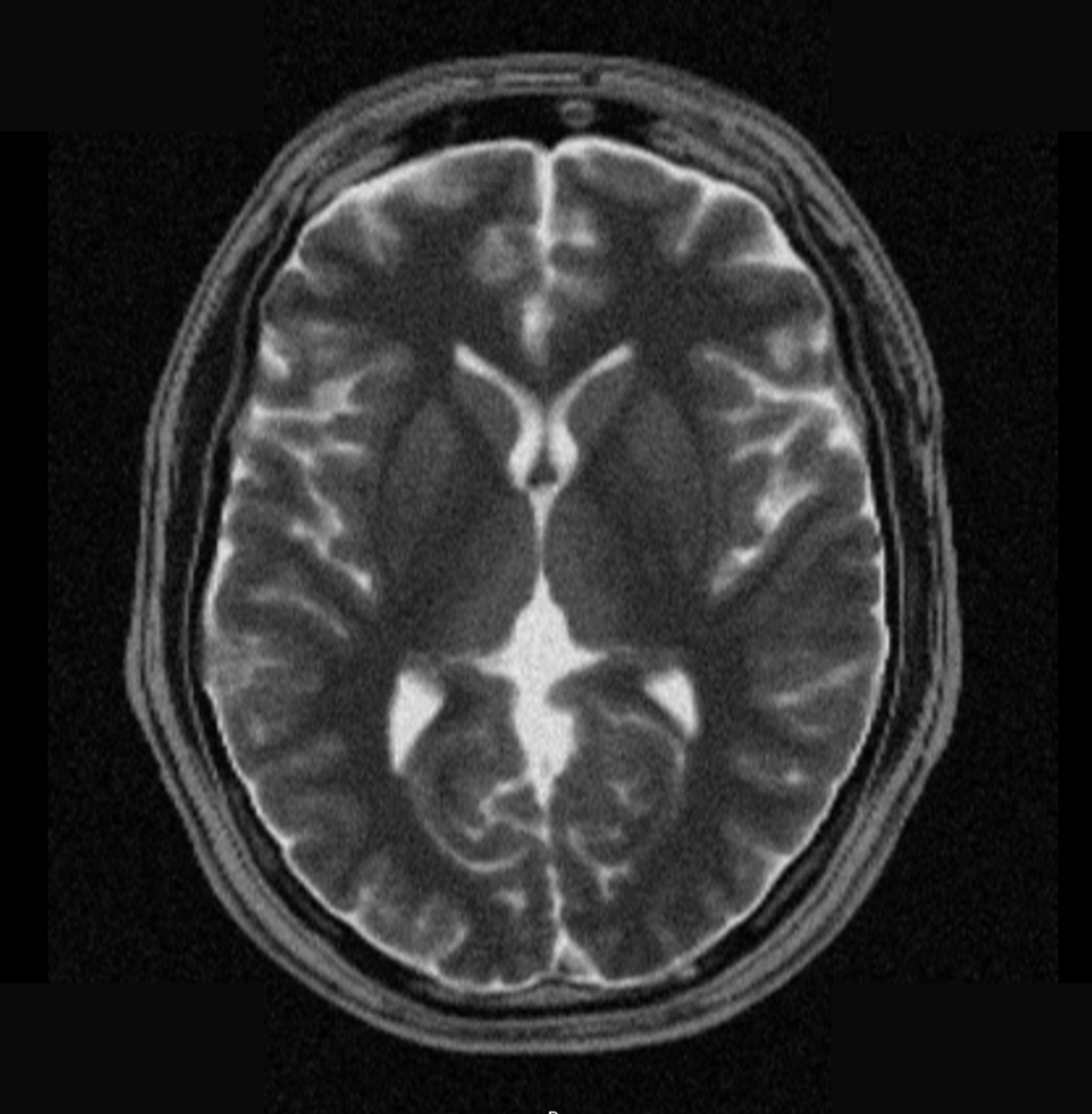
T2-Weighted Images – Highlight Fluid-Related Tissues and Conditions
T2-weighted imaging makes fluids appear bright. This contrast is ideal for detecting tissues and abnormalities associated with high water content.
In brain MRI, T2 sequences are excellent for evaluating hydrocephalus, cysts, and edema. They clearly show the ventricles and cerebrospinal fluid spaces, making them useful for assessing size and configuration of these structures.
✅ Axial T2 of the Brain – Correct Image:
The axial T2 sequence provides a horizontal view of the brain, which lets us:
Assess the ventricles for size and symmetry.
Evaluate brain parenchyma for areas of abnormal signal intensity.
Identify fluid collections such as cysts or edema.
Visualize the basal ganglia and other deep brain structures.
T2 FLAIR – Best for White Matter Lesions
T2 FLAIR (Fluid Attenuated Inversion Recovery) is a special type of T2-weighted sequence that suppresses the signal from cerebrospinal fluid (CSF), making it appear dark instead of bright. This makes it the best sequence in the protocol for lesions sitting next to CSF spaces.
In brain MRI, FLAIR sequences are important for evaluating multiple sclerosis, small vessel disease, and chronic ischemia. They are particularly effective at highlighting white matter lesions near the ventricles.
✅ Axial T2 FLAIR of the Brain – Correct Image:
The axial T2 FLAIR sequence provides a view similar to T2, but with CSF suppression, which lets us:
Detect periventricular white matter lesions more clearly without interference from bright CSF.
Evaluate areas of edema which remain bright against the dark CSF background.
Identify subtle abnormalities that might be overlooked on standard T2 images.
T1-Weighted MRI – Key for Gray-White Matter Contrast and Post-Contrast Scans
T1-weighted imaging makes fat appear bright and fluid dark. That combination is what makes it useful for fat-rich tissue and for structural detail.
In brain MRI, T1 sequences are used to evaluate structural anatomy, tumors, metastases, and subacute hemorrhage. They provide excellent contrast between gray and white matter, and serve as the baseline for post-contrast studies.
✅ Axial T1 of the Brain – Correct Image:
The axial T1 sequence provides a horizontal view, showing:
Clear differentiation between gray and white matter.
Anatomical details of brain structures.
Fat-containing structures appear bright, helping to identify normal and abnormal fat distribution.
✅ Sagittal T1 of the Brain – Correct Image:
The sagittal T1 sequence provides a side view of the brain, which lets us:
Evaluate midline structures such as the corpus callosum, brainstem, and cerebellum.
Assess the pituitary gland and sella turcica.
Visualize the ventricles from a different perspective.
✅ Coronal T1 of the Brain – Correct Image:
The coronal T1 sequence provides a front-to-back view, useful for:
Comparing left and right hemispheres side by side to check for symmetry.
Evaluating the temporal lobes and hippocampus.
Assessing the ventricular system from an alternative angle.
Diffusion-Weighted Imaging (DWI) – Best for Acute Stroke
Diffusion-weighted imaging is sensitive to the movement of water molecules in tissue. In normal brain tissue, water diffuses freely, but in damaged areas such as an acute stroke, water movement is restricted.
In brain MRI, DWI is the key technique for evaluating acute stroke and cytotoxic edema. It can reveal ischemic changes within minutes of onset, far earlier than the other sequences, which is what makes it the first sequence read in a suspected stroke. An early negative DWI does not rule stroke out on its own.
The DWI sequence generates 3 different types of images from a single series, each providing unique diagnostic information:
1. b=0 Image – The Unweighted Reference
The b=0 image is acquired at the start of the diffusion sequence with no diffusion gradients applied. It is effectively a T2-weighted EPI image showing baseline tissue contrast before any diffusion weighting.
It serves two purposes:
Provides the anatomical and signal reference that the ADC map is calculated against.
Shows how much of the brightness on the b=1000 image comes from T2 effects rather than from restricted diffusion, which is what T2 shine-through means.
Because it is an EPI readout with no diffusion gradients, this is also the image where susceptibility effects near air-tissue interfaces and metal are easiest to spot. Some departments read it specifically to look for blood products, which is where the informal name comes from. It is still the b=0 acquisition rather than a computed susceptibility map, and on its own it cannot correct geometric distortion, which needs either a field map or a second acquisition with reversed phase-encode polarity.
✅ Correct Image Example:
2. Trace DWI Image (b=1000)
The trace image at b=1000 shows areas of restricted water diffusion as bright signal. It is diffusion weighted rather than a measurement of diffusion, which is why restriction is only confirmed when bright signal here is matched by dark signal on the ADC map.
This is the primary image for identifying acute stroke, showing the infarct core as a hyperintense (bright) region within minutes of symptom onset.
✅ Correct Image Example:
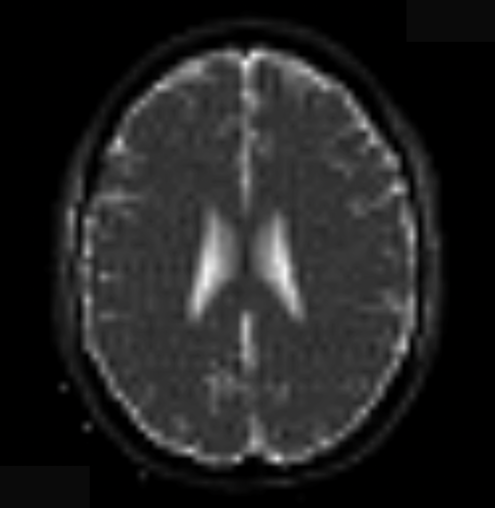
3. ADC Map (Apparent Diffusion Coefficient)
The ADC (Apparent Diffusion Coefficient) Map quantifies the degree of water diffusion, where restricted diffusion appears dark.
The map shows whether bright areas on the DWI come from genuinely restricted water movement, as in acute stroke, or only from tissue that is already bright on T2-weighted images, which is called T2 shine-through. This distinction decides the diagnosis.
The map also separates acute ischemia from subacute and chronic lesions. Acute stroke appears dark on ADC maps, while chronic lesions typically show normal or increased diffusion.
✅ Correct Image Example:
When these three DWI images are evaluated together, they provide comprehensive information about water diffusion in brain tissue.
This enables accurate diagnosis of acute ischemia and lets us differentiate it from other pathologies that appear similar on standard sequences.
Final Checks:
Before finishing a brain MRI, always check these 6 points to ensure diagnostic quality:
Symmetry: Brain structures on both sides must appear symmetric and scroll together across slices; asymmetry may suggest pathology or poor positioning.
Full Coverage: Slices must extend from the vertex to the base of the skull, covering cortex, ventricles, brainstem, and cerebellum.
Gray-White Matter Contrast: T1 and T2 images must clearly show differentiation between gray and white matter for structural evaluation.
CSF Suppression on FLAIR: T2 FLAIR must show dark CSF; bright signal here may indicate poor suppression or incorrect TI.
DWI and ADC Agreement: Acute stroke appears bright on DWI and dark on ADC; mismatches may signal T2 shine-through or artifact.
Image Quality and Artifacts: All sequences must have strong SNR, sharp detail, and no motion, wrap-around, or ghosting artifacts.
By following this protocol and carefully reviewing the images, you can ensure an excellent diagnostic evaluation of the brain.

.svg)