How to plan a cardiac MRI viability protocol (Part 2)

This step-by-step guide is for MRI students, radiographers and technologists who wish to improve their planning skills and master the cardiac viability MRI protocol.

This guide is Part 2 of a cardiac viability assessment. In Part 1, we covered cardiac morphology and function.

In this Part 2, we will follow up with tissue characterization, where we determine which damaged parts of the myocardium can recover with treatment, and which are permanently scarred.

What you will learn:

1. Patient and scanner setup tips.
2. How to perform perfusion, early, and late gadolinium enhancement.
3. What parameters optimize tissue characterization.
4. Ways to avoid common contrast protocol errors.
5. How to identify viable vs non-viable myocardium.

In Part 1 of our cardiac viability protocol, we completed all function and morphology sequences. We captured the heart's pumping action with cine images and checked for structural abnormalities with black and bright blood sequences.

Now we continue with another core part of viability assessment: tissue characterization. This is where we determine which damaged heart areas can recover with treatment, and which are permanently scarred.

The scar itself never regains function. What matters is how much healthy muscle is left around it.

A small scar leaves healthy muscle behind. That muscle can recover after revascularization procedures like bypass surgery or stenting.

A scar through the full wall leaves no healthy muscle behind. There is nothing left to recover.

How to Balance the 3 Trade-offs in Cardiac Viability MRIs

In MRI, we always face a trade-off between 3 key metrics:

1. Scan Time: How fast a pulse sequence can be completed.
2. Resolution: How much detail the image can display.
3. SNR: How clear the image is, how much signal relative to noise.

Improving one of these metrics reduces the performance of the others. To decide what trade-offs to make, we must consider the needs of each clinical situation.

In cardiac viability MRIs:

• The main goal is to clearly distinguish between scarred and healthy heart muscle.
• The depth and extent of damage can be just 1–2 mm, so we also need good resolution.
• Scan time matters, but we can often afford a bit more time if the patient can cooperate.

Therefore, we typically:

1. Prioritize SNR to clearly distinguish scarred tissue from healthy myocardium, which is the whole point of viability imaging.
2. Maintain enough resolution to assess scar depth, since the extent of damage can be just 1-2 mm.
3. Optimize scan time last, keeping it practical, since patients undergoing viability imaging can generally cooperate with a somewhat longer scan.

This balance ensures we clearly see bright scar tissue against the dark, viable myocardium, which is the whole point of viability imaging.

How Contrast Enhancement Works in Cardiac MRI

Cardiac tissue characterization can be done either with or without contrast.

Without contrast, we use mapping sequences like T1, T2, or T2* to assess tissue properties.

With contrast, we give the patient a single bolus of gadolinium (Dotarem or Gadovist). Then, we capture images at three specific time points:

1. Perfusion: Immediately as contrast arrives (0–1 minute)
2. Early Enhancement: At 2–4 minutes after injection
3. Late Enhancement: At 10–15 minutes after injection

Each phase reveals different pathology because of how contrast behaves in healthy vs damaged tissue. The following section shows which health conditions each sequence detects.

Health Conditions in Cardiac Tissue Viability – And the MRI Sequences That Reveal Them

The table below lists some of the most common cardiac conditions related to tissue characterization:

The step-by-step guide below will show you how to set up and perform contrast-enhanced tissue characterization, which is the second part of a complete viability assessment.

We will perform the protocol in 3 parts:

1. Inject the Contrast Agent
2. Plan and Acquire the Protocol Sequences
3. Review the Images

Step 1: Inject the Contrast Agent

1. Verify That It’s Safe to Do a Contrast Injection

Before any contrast injection, you must verify that the patient can handle it. Their eGFR must be above 30 mL/min/1.73 m², but check your hospital's specific cutoff.

If the patient’s kidneys can't handle the contrast safely, either perform non-contrast tissue characterization or end the exam. Never compromise patient safety for imaging.

2. Prepare and Administer the Contrast Injection

Follow these steps to ensure you prepare and administer the contrast injection correctly:

Step 2: Plan and Acquire the Protocol Sequences

When all preparations are ready, we can start planning and acquiring the protocol sequences.

Let's go through the pulse sequences a standard cardiac tissue viability MRI protocol includes, why we perform them, and how to set them up.

The 9 Sequences of a Standard Cardiac Tissue Viability Protocol

1. SAX Perfusion GRE (Gradient Echo)
2. 4-chamber Early Enhancement IR-GRE (Inversion Recovery GRE)
3. 2-chamber Early Enhancement IR-GRE
4. 3-chamber Early Enhancement IR-GRE
5. SAX TI Scout
6. 4-chamber Late Enhancement IR-GRE
7. 2-chamber Late Enhancement IR-GRE
8. 3-chamber Late Enhancement IR-GRE
9. SAX Late Enhancement IR-GRE

We mainly use Inversion Recovery Gradient Echo (IR-GRE) sequences for this study. This type of sequence makes scarred tissue appear bright, while normal heart muscle appears dark, which makes it easy to spot areas of scarred heart muscle.

These sequences also work with ECG-gating to take pictures between heartbeats, which reduces blurring from heart motion and gives clearer images.

The protocol follows this timeline:

1. Baseline perfusion images (8–10 phases before contrast)
2. Inject contrast and continue perfusion (45–50 more phases)
3. Early enhancement at 2–4 minutes (4ch, 2ch, 3ch)
4. TI Scout immediately before late enhancement, around 10–15 minutes
5. Late enhancement at 10–15 minutes (4ch, 2ch, 3ch, SAX)

In the sections below, we go through how to plan and set up each sequence.

1. Short-Axis (SAX) Perfusion GRE

The perfusion sequence tracks contrast as it flows through the heart muscle. This sequence captures 3 short-axis slices at basal, mid and apical level. It samples the left ventricle at three levels rather than covering it continuously, so perfusion defects between the sampled levels are not shown. The late enhancement short-axis stack is what covers the ventricle in full.

This viability protocol uses rest perfusion only. No vasodilator such as adenosine or regadenoson is given, because the goal is to map established damage rather than to test for inducible ischemia.

Start the perfusion sequence and acquire 8–10 baseline images. Then inject contrast and capture another 45–50 phases as it washes through.

Watch for the contrast arriving in the right ventricle first, then left ventricle, then myocardium. Normal tissue enhances uniformly. Dark areas indicate perfusion defects.

For patients with poor cardiac function, increase phases to 80–100. The slow-moving heart needs more time points to capture the full contrast passage.

✅ Correct Planning:

Planning Instructions:

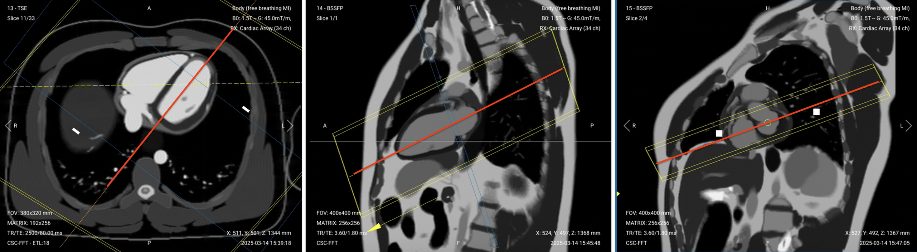
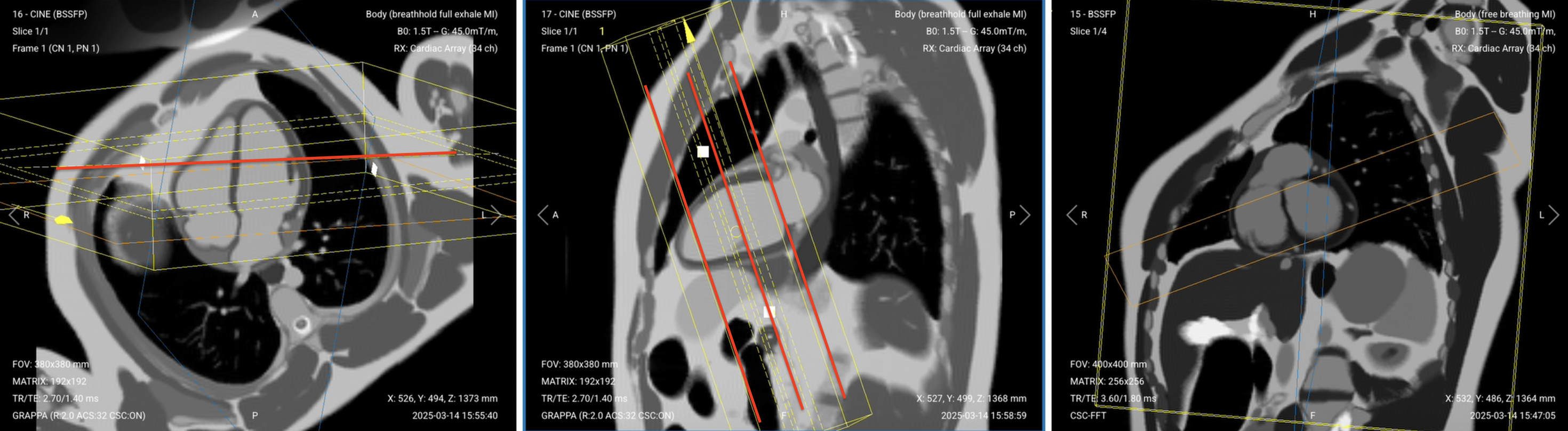
• Plan the stack using the 2-chamber cine and 4-chamber cine views.
• Use the left ventricle and mitral valve as your anatomical references.
• Align the slices as follows:
  • 2-chamber cine: Position slices perpendicular to the long axis of the left ventricle. Space them evenly from base to apex.
  • 4-chamber cine: Ensure slices are perpendicular to the interventricular septum and cover the full left ventricle.
• Use appropriate geometry parameters:
  • Slice number: 3 slices (basal, mid, apical) to cover key myocardial regions.
  • Slice thickness: 8–10 mm for adequate coverage with good SNR.
  • Slice gap: 8–10 mm between slices to avoid overlap while covering the full ventricle.
• Set the fold-over direction (phase encoding) to anterior-to-posterior (AP) to minimize wrap artifacts from the lateral chest.

Parameters for Short-Axis (SAX) Perfusion:

The sequence uses a saturation preparation rather than an inversion, which is what makes signal track contrast concentration during the first pass. Acquire enough time points to follow the whole first pass, typically 50 to 60 for normal function and 80 to 100 where the heart pumps slowly.

2. Early Enhancement Sequences (IR-GRE)

Early enhancement shows microvascular obstruction (MVO). These are areas where contrast can't penetrate due to severe acute damage.

Set up three views (4ch, 2ch, 3ch) with very high TI (~440 ms) to make both blood and normal myocardium bright. Any dark spots indicate MVO.

Run these sequences immediately after perfusion finishes, about 2–4 minutes after injection. If you do a manual injection, wait a bit longer (3–4 minutes) since hand-pushing is slower than power injectors.

In healthy patients, both myocardium and blood pool should appear bright. Dark spots within bright myocardium indicate microvascular obstruction, i.e. fresh damage where vessels are blocked.

Planning Instructions:

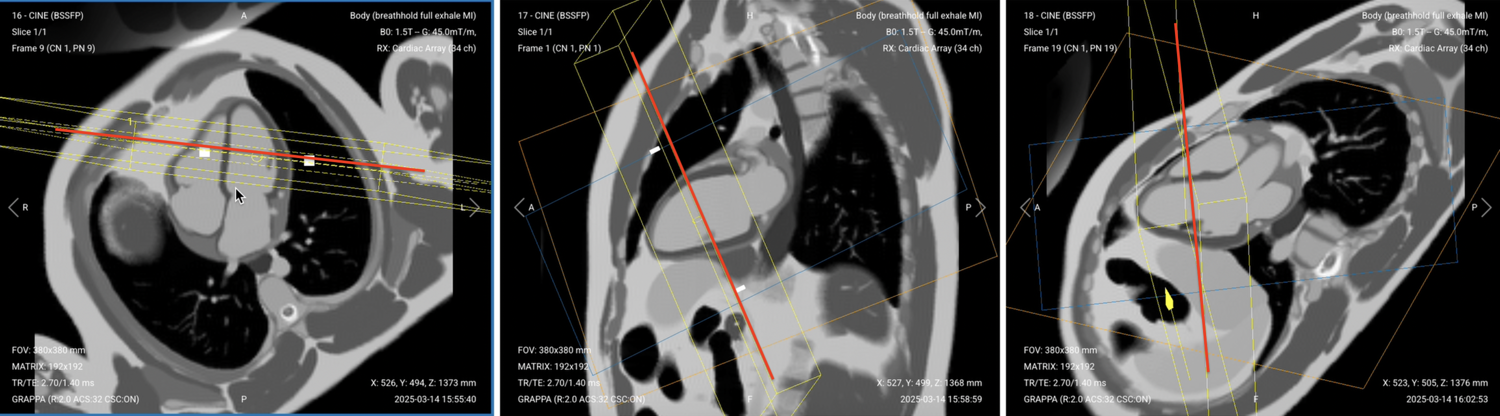
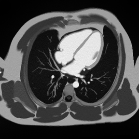
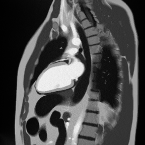
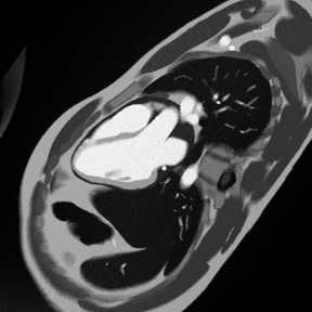
• Copy the slice geometry and planning from the corresponding cine sequences (4ch, 2ch, 3ch).
• Keep identical positioning to enable direct comparison with function images.

✅ Correct Planning for 4-Chamber Early Enhancement:

✅ Correct Planning for 2-Chamber Early Enhancement:

✅ Correct Planning for 3-Chamber Early Enhancement:

Parameters for Early Enhancement (All Views):

The acquisition is gated to the quiet part of the cardiac cycle, which is what keeps scar borders sharp.

3. TI Scout – Finding the Myocardium Null Point

The TI Scout sequence shows multiple images with different inversion times. The goal is to find the exact timing that nulls healthy myocardium so it appears completely black.

The TI value from this image (typically 200–250 ms at 1.5 T) will be used for all late enhancement sequences.

Run the TI Scout immediately before the late enhancement series, at roughly 10 to 15 minutes after injection, so the null point it reports still applies when the diagnostic images are acquired.

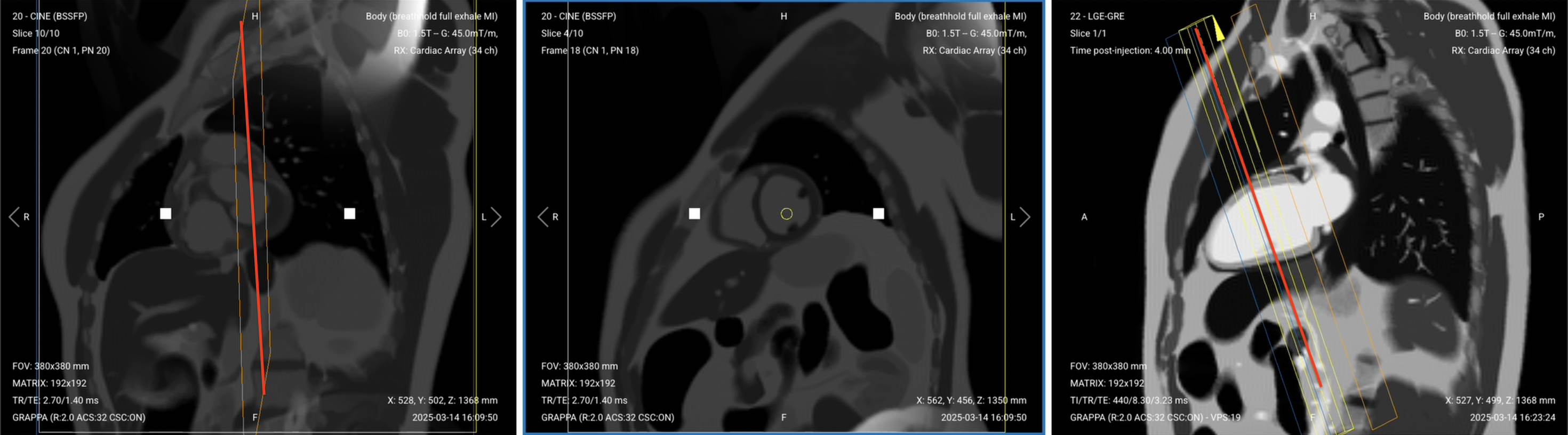
✅ Correct Planning:

Planning Instructions:

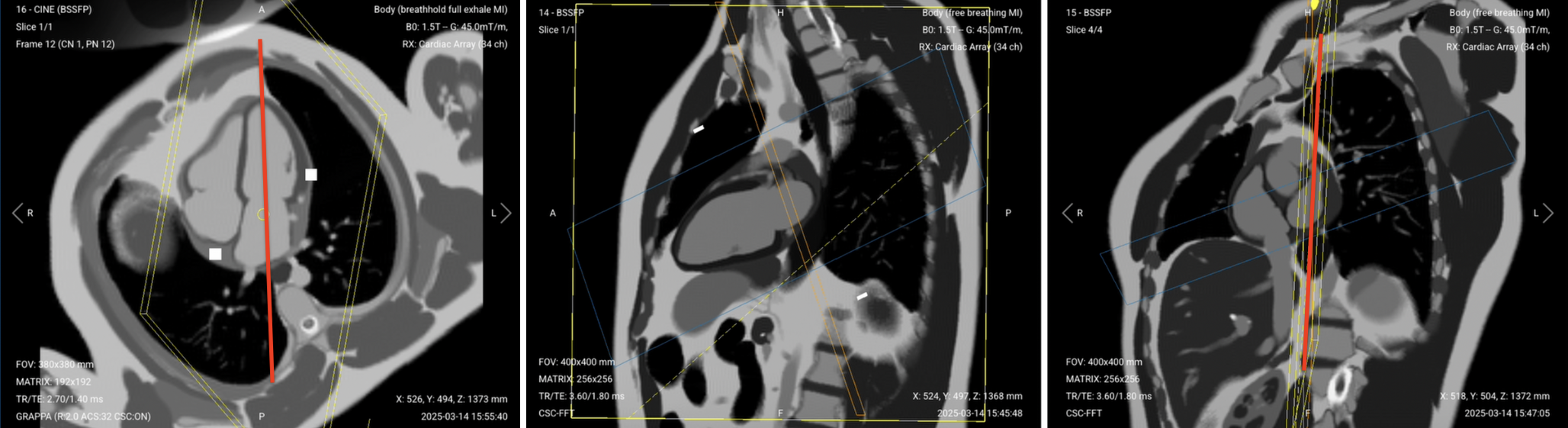
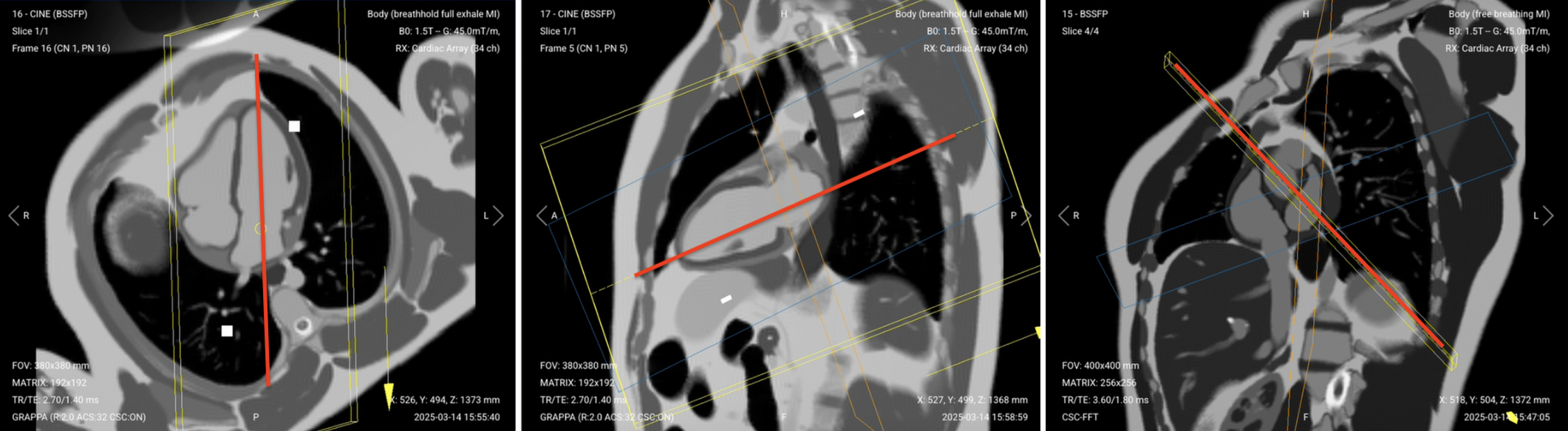
• Copy the slice geometry and planning from your previous SAX cine stack. Start by scrolling through the cine slices and select a mid-ventricular slice to copy; a slice that shows a full ring of myocardium.
• Use the left ventricle as your anatomical reference.
• In the long-axis view, center on the left ventricle at the papillary muscle level.
• Use appropriate geometry parameters:
  • Slice number: 1 slice at mid-ventricular level.
  • Slice thickness: 8 mm for good SNR during multiple TI sampling.
  • Slice gap: Not applicable (single slice).
• Set the fold-over direction (phase encoding) to foot-head (FH), matching the short-axis cine stack.

Parameters for TI Scout:

How to Read the TI Scout to Find the Right TI Value

Once your TI Scout has finished running, we must now read the resulting images to find the right TI value.

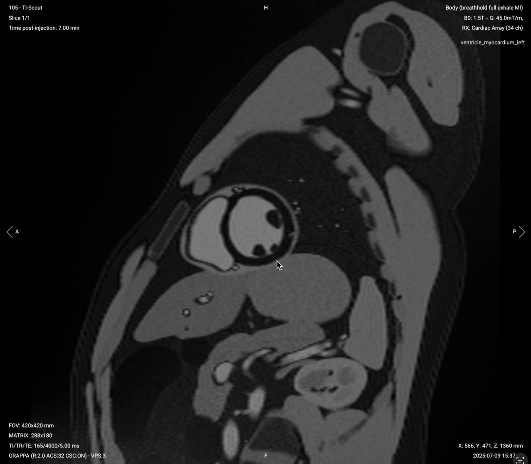
The scout starts at a short inversion time and steps upward across the series, so scrolling through the images shows the myocardium darken, null, then brighten again. Read the null point off the image where the myocardium is darkest and the epicardium is still visible.

Scroll through its images and look at the areas where 1) the myocardium interfaces with the blood pool, and 2) the papillary muscles and epicardium cross over.

✅ TI Scout – Correct Image Example:

In these areas, look for these key features:

• Myocardium appears darkest
• Epicardium can be clearly seen as a bright line (but not too bright)
• Chest wall muscles also dark (confirming proper muscle nulling)
• Clear distinction between nulled myocardium and bright blood pool

The correct TI for late enhancement typically falls between 200–250 ms at 10–15 minutes post-contrast. Select the value that best nulls the myocardium.

The null point drifts upward as contrast continues to wash out, so if the myocardium stops nulling cleanly on the later views, raise the TI slightly or repeat the scout.

4. Late Enhancement Sequences (IR-GRE)

Late gadolinium enhancement (LGE) is the gold standard for identifying myocardial scar. We acquire the same views as early enhancement but with an optimized TI to null healthy muscle.

Use the TI value from your scout to acquire all late enhancement sequences.

Planning Instructions for All Late Enhancement Views:

• Copy the slice geometry and planning from the corresponding cine sequences (4ch, 2ch, 3ch).
• For the short-axis stack, copy the slice geometry, slice count and foldover direction from the short-axis cine stack, so the two stacks align segment by segment for AHA scoring.
• Keep identical positioning to enable direct comparison with function images.
• Set TI based on the TI Scout result (typically 200–250 ms).

✅ Correct Planning for 4-Chamber Late Enhancement (same as early 4-chamber):

✅ Correct Planning for 2-Chamber Late Enhancement (same as early 2-chamber):

✅ Correct Planning for 3-Chamber Late Enhancement (same as early 3-chamber):

✅ Correct Planning for SAX Late Enhancement:

Parameters for Late Enhancement (Long-Axis Views):

Parameters for Late Enhancement (Short-Axis Stack):

5 Common Mistakes in Cardiac Contrast Enhancement and How to Avoid Them

Mistake 1: Incorrect Inversion Time (TI)

Late gadolinium enhancement only works if the TI is set to fully null the signal from healthy myocardium. Using the wrong value may cause scars to appear faint or blend in with normal tissue.

To get reliable results, always run a TI Scout first and select the recommended time, which is typically 200–250 ms.

Mistake 2: Mismatched Slice Planning

Late enhancement images are meant to be compared directly with cine views from the function study. But if slice plannings don’t match, those comparisons lose value.

You should thus always copy the exact slice positions from your cine sequences for each view, including the 4-chamber, 2-chamber, 3-chamber, and short axis.

Mistake 3: Planning Sequences After Injecting Contrast

Timing is critical once contrast is administered, since each phase must be captured at the right moment.

To keep everything on schedule, all sequences must be fully prepared and positioned before the injection begins.

Mistake 4: Too Few Phases in Perfusion Imaging

Perfusion sequences capture the passage of contrast through the myocardium in real time, so you need enough temporal resolution to follow the entire flow. If the heart is pumping slowly, short sequences may miss part of the wash-in.

Use 50–60 phases as a baseline for patients with normal cardiac function. If the cine images showed sluggish motion, increase to 80–100 phases to capture the full contrast passage.

Mistake 5: Skipping Patient Safety Check Before Contrast

Gadolinium contrast can pose serious risks for patients with impaired kidney function.

Always confirm that the patient’s eGFR is above 30, or your site’s official threshold, before proceeding with any contrast-enhanced sequences. Choose non-contrast options if the patient isn’t cleared.

Step 3: Review the Images

Finally, we will review the images to ensure all the anatomical information we need is clear.

In a cardiac viability tissue characterization MRI, these structures must be clearly visible:

1. Myocardial scar tissue, including transmural extent and subendocardial involvement
2. Microvascular obstruction (MVO) zones within infarcted areas
3. Viable myocardium with normal nulling on late enhancement
4. Left ventricular walls in all 17 segments per AHA model
5. Papillary muscles and their enhancement patterns
6. Pericardium and any pericardial enhancement

Below, we will go through all the different image contrasts and explain their specific role in tissue characterization.

Perfusion Gradient Echo – Shows Blood Flow Through the Myocardium as Contrast Arrives

Perfusion imaging captures the first pass of contrast agent through the heart muscle. As contrast arrives, normal myocardium enhances quickly and evenly. Areas with poor blood flow remain dark.

In cardiac viability, rest perfusion identifies areas of reduced blood flow caused by scar tissue or ischemia. Dark regions during first-pass indicate either infarcted tissue or severely narrowed arteries.

The contrast between dark under-perfused tissue and bright normally perfused myocardium helps determine:

• Defect size and location
• Transmural extent (how deep the defect goes)
• Viability for revascularization: whether the myocardium is viable or permanently scarred

We capture perfusion in short-axis views at basal, mid, and apical levels to assess the entire left ventricle.

✅ Short-Axis Rest Perfusion Gradient Echo – Correct Image Example:

In the frame below, we can see a perfusion defect. This is the black semi-circle border that stretches the top-half of the left ventricle. (The left ventricle is shown on the right side in this image).

As labeled on the image, the thinner rim is likely a subendocardial scar, involving less than 50% of wall thickness, and the thicker rim is likely a transmural scar, covering the full wall thickness. Perfusion alone cannot confirm which is which; the late enhancement images establish the actual transmural extent.

Things to Look for in Rest Perfusion:

• Dark areas that persist throughout contrast arrival indicate perfusion defects
• Normal myocardium should enhance uniformly within 1–2 heartbeats
• A persistent subendocardial rest-perfusion defect is abnormal but not specific. Compare it with the late enhancement images and the clinical history.
• Transmural defects indicate more severe disease or infarction

Early Gadolinium Enhancement – Reveals Acute Injury and Microvascular Obstruction

Early enhancement sequences are acquired 2–4 minutes after contrast injection. At this timing, contrast has entered most tissues but hasn't yet penetrated areas with microvascular obstruction (MVO).

MVO appears as dark zones within bright infarcted tissue. This represents severe microvascular damage where even contrast molecules can't penetrate. Finding MVO is important because it predicts worse outcomes and larger final infarct size.

We acquire early enhancement in 4-chamber, 2-chamber, and 3-chamber views to see MVO from multiple angles.

✅ 4-Chamber Early Gadolinium Enhancement – Correct Image Example:

Things to Look for in 4-Chamber Early Enhancement:

• Assess all visible walls for dark MVO zones
• Both ventricles should be clearly visible
• Look for any pericardial enhancement suggesting inflammation

✅ 2-Chamber Early Gadolinium Enhancement – Correct Image Example:

Things to Look for in 2-Chamber Early Enhancement:

• Dark zones within bright areas indicate MVO
• Both blood pool and myocardium should appear bright
• MVO typically occurs in the core of large infarcts
• Size and location help predict recovery potential

✅ 3-Chamber Early Gadolinium Enhancement – Correct Image Example:

Things to Look for in 3-Chamber Early Enhancement:

• Check the septum and inferior wall for MVO
• Ensure the aortic outflow tract is visible
• Compare with late enhancement to track MVO evolution

Late Gadolinium Enhancement (LGE) – The Gold Standard for Scar Detection

Late enhancement imaging takes place 10–15 minutes after contrast injection. By this time, contrast has washed out of normal myocardium but remains trapped in scar tissue.

This sequence answers the central clinical question:

“How much of the heart muscle is permanently damaged?”

To highlight scar tissue clearly, we use the TI Scout to select the correct inversion time (TI) that nulls the signal from healthy myocardium. When done correctly, healthy muscle appears dark, while scar tissue stands out as bright white.

The amount of scar tells us how likely the tissue is to recover after treatment:

Transmural extent is how much of the wall thickness has scarred. It is reported in bands: 0%, 1–25%, 26–50%, 51–75% and 76–100%. The larger the share, the less healthy muscle remains and the less likely the segment is to recover.

Enhancement below about 50% of wall thickness is subendocardial. Like toast burnt on one side only, it may still be salvageable. Enhancement above about 50%, reaching all the way to the epicardium, is transmural. Like toast burnt all the way through, it is unlikely to recover.

To fully understand the location and depth of scarring, we acquire late enhancement images in multiple views.

✅ 4-Chamber LGE – Correct Image Example:

Things to Look for in 4-Chamber LGE:

• Evaluate all four chambers for abnormal enhancement
• Enhancement at the right ventricular insertion points is a recognized non-ischemic pattern rather than an infarct, since it does not follow a coronary territory. Record it rather than treating it as incidental, and do not read it as scar.
• Check for thrombus (appears dark) adjacent to scar

✅ 2-Chamber LGE – Correct Image Example:

Things to Look for in 2-Chamber Late Enhancement:

• Bright areas indicate scar tissue
• Measure transmural extent (percentage of wall thickness)
• Subendocardial scars appear as bright inner rim
• Check inferior and anterior walls

✅ 3-Chamber LGE – Correct Image Example:

Things to Look for in 3-Chamber Late Enhancement:

• Assess basal septum and inferolateral wall
• Look for scar extension into papillary muscles
• Ensure proper nulling of normal myocardium

✅ SAX LGE – Correct Image Example:

Things to Look for in SAX LGE:

• Systematically assess all 17 AHA segments
• Document scar location, size, and transmural extent
• Compare with perfusion defects to identify hibernating myocardium
• Look for papillary muscle involvement

Final Checks:

Before finishing a cardiac viability tissue characterization MRI, always check these 5 points to ensure diagnostic quality:

1. Complete Coverage: The late enhancement short-axis stack runs from base to apex with no gaps. Perfusion covers basal, mid and apical levels. Early enhancement covers the 4-chamber, 2-chamber and 3-chamber views.
2. Proper Nulling: Normal myocardium appears uniformly black on late enhancement with TI verified by scout sequence.
3. Scar Assessment: Transmural extent clearly visible and measurable in all affected segments.
4. MVO Detection: Early enhancement sequences checked for dark zones within infarcted areas.
5. Image Quality: All sequences have adequate SNR, sharp borders, and minimal artifacts from arrhythmias or breathing.