How to plan an ankle MRI protocol with metal implant
Written by:
Erik Jacobsson
This step-by-step guide is for MRI students, radiographers, and technologists who wish to improve their planning skills and master the ankle MRI protocol with metal implants.
What you will learn:
Key factors in ankle MRIs with metal implants, including trade-offs.
Patient and scanner setup tips.
Best pulse sequences and planning techniques.
Ways to avoid common artifacts.
What great images of ankles with metal implants should look like.
Key Takeaways
Because metal implants create artifacts that hide anatomy, it's recommended to prioritize resolution.
Metal artifacts can obscure important structures around the implant. We need high resolution to see tissues clearly and strong SNR to overcome signal loss from the metal.
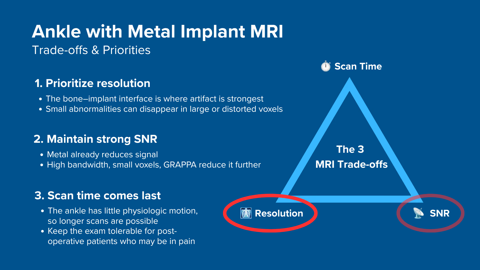
Therefore, we typically 1) prioritize resolution, 2) maintain strong SNR, and 3) optimize scan time as needed.
For ankle MRIs with implants, we mainly use Turbo Spin Echo with STIR fat suppression.
Turbo Spin Echo (TSE) handles metal artifacts far better than gradient echo sequences. STIR fat suppression also works better than spectral suppression around metal, because it doesn't rely on a uniform magnetic field.
This combination of TSE + STIR helps us see tissues around implants clearly to check for infection, loosening, or healing problems.
Avoid these 5 common ankle artifacts when imaging with metal implants.
Artifacts
Solution – How to Avoid It
Metal artifacts
Increase bandwidth per pixel, use small voxels and thin slices, keep TE short, and choose TSE over gradient echo.
Chemical shift artifacts
Increase the bandwidth above 220 Hz per pixel at 1.5 T, and roughly double that at 3 T.
Wrap-around artifacts
Set appropriate phase direction and use foldover suppression.
Motion artifacts
Shorten scan time to reduce motion blur.
Flow artifacts
Adjust the phase-encoding direction so ghosting does not cross the bone-implant interface, or use flow compensation if available.
Intro to Ankle MRIs with Metal Implants
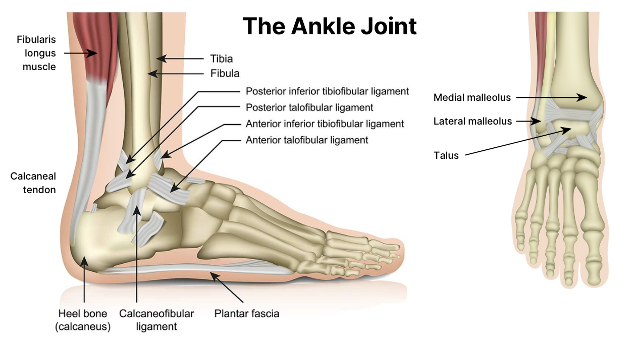
The ankle is a complex joint that handles a lot of pressure. It supports our full body weight daily through walking, running, and jumping.
Due to high stress and frequent injuries, many patients receive metal implants for fracture fixation, joint replacement, or ligament reconstruction.
When imaging ankles with metal implants, however, we face unique challenges. Metal disrupts the magnetic field and creates artifacts that can hide important anatomy.
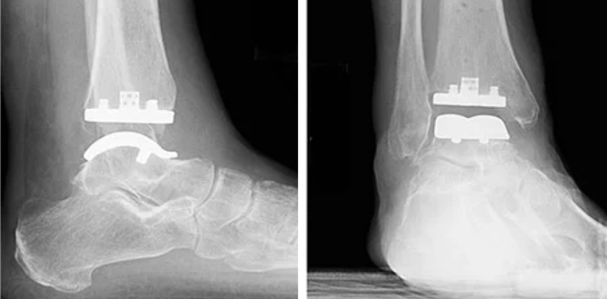
Implant of a total ankle replacement, seen from lateral (side view) and anteroposterior (front view). X-ray images. Image credit: Hospital for Special Surgery
We must therefore use special techniques to handle these metal artifacts.
Implant Materials and MR Safety Labeling
Most orthopedic implants are made from one of three materials:
Polymers
Ceramics
Metals
MR labeling attaches to the finished device, not to a material. A device is MR Safe, MR Conditional or MR Unsafe because it was tested and labeled that way, and no material name settles the question on its own.
Pure polymer and ceramic components, such as plastic spacers and ceramic heads, are typically labeled MR Safe. They are not magnetic, they do not conduct current, and they do not distort the magnetic field. They still appear as a signal void, because they contain no mobile protons.
Many implants are composite constructions, for example a ceramic head on a metal stem, or a PEEK cage with titanium markers. Judge the labeled device, never the material.
Metals are different. While they may be weakly or non-magnetic, they can still disrupt image quality. This is why most metal implants are labeled "MR Conditional". They are safe to scan under specific conditions, but they may cause artifacts.
Before scanning, always:
Ask the patient if they have any implants.
Request implant documentation when available.
Check implant safety on resources like MRIsafety.com.
There are three labeling categories to know:
MR Safe means the item poses no known hazard in any MR environment.
MR Conditional means it is safe under specified conditions, such as a stated field strength and SAR limit.
MR Unsafe means it must not enter the scanner room.
Once confirmed as MR Safe or MR Conditional, the focus shifts to managing image quality and safety.
How Different Metals Affect Image Quality and Patient Safety
Even when an implant is MR Conditional and safe to scan under the stated conditions, it can still degrade image quality.
How severe the artifact is depends on the metal's magnetic susceptibility, meaning how much it perturbs the surrounding magnetic field compared to tissue. Some metals, like stainless steel and cobalt-chromium, cause significant artifacts that distort or hide anatomy.
Other metals, like titanium and tantalum, have minimal impact.
Note: Stainless steel is itself an iron alloy. The surgical grades used in modern implants, such as 316L, are austenitic and only weakly magnetic. Older carbon steel and martensitic grades are ferromagnetic and produce far more severe artifact.
Implants can also heat surrounding tissue when radiofrequency pulses induce electrical currents in the metal. Around the ankle this is most relevant for hardware such as intramedullary tibial nails, long fixation plates and external fixator components. Heating risk depends on the device's geometry, material and position as well as on the sequence, so follow the conditions stated in the device labeling rather than judging by size alone.
To reduce heating risk:
Avoid sequences with high Specific Absorption Rate (SAR).
Limit scan duration where possible.
Monitor the patient closely during the exam.
MARS vs SMART: The 2 Approaches to Metal Implant Imaging
Once an implant is cleared for scanning, the next step is choosing how to reduce artifacts. There are two main approaches:
MARS – Metal Artifact Reduction Sequences
MARS uses prebuilt sequences developed by scanner vendors. These are built on spin echo acquisitions combined with vendor-specific correction methods, such as View Angle Tilting, slice-encoding correction, or multispectral acquisition. The three implementations below differ in what they correct, so results are not interchangeable.
Each vendor has their own version of MARS:
Siemens: WARP
GE: MAVRIC
Philips: O-MAR
The benefit of MARS is that they are pre-configured and are ready to scan. You simply select the preset and adjust a few parameters.
However, each version of MARS is vendor-specific and is not available on other scanners.
SMART – Standard Metal Artifact Reduction Techniques
In this guide, "SMART" is our teaching label for standard parameter-based metal artifact reduction, not an industry-standard term. The techniques themselves are standard; the acronym is ours.
SMART uses regular turbo spin echo sequences that are available on any scanner to control metal artifacts and manage the resulting scan time, such as:
Increasing spatial resolution
Raising bandwidth above 220 Hz/pixel
Enabling GRAPPA or other parallel imaging
SMART therefore takes more work to set up. However, you can use the same SMART sequences on any scanner, regardless of brand.
This approach gives you full control, and the principles transfer to any scanner. The exact settings and the resulting images remain vendor and scanner dependent, so expect to re-tune the numbers on each system.
The Parameters We Adjust Most in This Protocol
To handle metal artifacts with the SMART approach, there are four key parameters we adjust.
Spatial resolution: Small voxels limit how much of the anatomy a single distorted voxel can swallow, and they are what let us assess the tissue immediately around the implant. This is the parameter we protect first.
Bandwidth per pixel: At 1.5 T, the fat and water resonances are about 220 Hz apart. Setting the bandwidth per pixel above that figure confines the fat-water misregistration to less than one pixel, so chemical shift stops being visible. Raising it further also shortens echo spacing, which limits how far the metal can distort the image geometry.
NEX/NSA/Averages: High bandwidth reduces SNR, so we must add more signal averages to get that signal strength back. This keeps our images clear while controlling metal artifacts.
Parallel imaging (GRAPPA): Skipping every second phase-encoding line and reconstructing the missing data from the coil elements halves the number of shots, which roughly halves the scan time. It also lowers SNR, so it is the second reason we raise the averages.
Other choices in this protocol also control metal artifact, including turbo spin echo rather than gradient echo, short TE, thin slices, and 1.5 T rather than 3 T. For severe distortion, vendor methods such as View Angle Tilting, slice-encoding correction or multispectral acquisition go further than parameter tuning alone.
How to Balance the 3 Trade-offs in Ankle MRIs with Metal Implants
In MRI, we always face a trade-off between 3 key metrics:
Scan Time: How fast a pulse sequence can be completed.
Resolution: How much detail the image can display.
SNR: How clear the image is, meaning how much signal we have compared with noise.
Improving one of these metrics often reduces the performance of the others. To decide what trade-offs to make, we must consider the needs of each clinical situation.
For ankle MRIs with metal implants, we face these challenges:
The tissue that matters, the bone-implant interface and the marrow right next to it, is exactly where the artifact is worst. A large voxel can swallow a thin rim of abnormal marrow completely.
Metal already reduces signal, and the settings that control its artifact cost more SNR on top of that: high bandwidth, small voxels, and GRAPPA all trade signal for less distortion.
The ankle tolerates a longer scan than most exams, since there's no breathing or cardiac motion. The real limit is the patient, since many are post-operative and in pain.
Therefore, we typically:
Prioritize resolution, since anatomy lost inside a distorted voxel generally cannot be recovered later in the exam.
Maintain enough SNR to keep that resolution diagnostic, buying it back with extra averages where the bandwidth and acceleration have taken it away.
Optimize scan time last, since this joint tolerates a longer acquisition, while keeping the total study short enough for a patient who may not manage a long one.
Note! Prioritizing resolution in ankle MRIs with metal implants is only a general guideline, NOT a strict rule. If your patient can't stay still for longer scans, you may need to reduce resolution slightly, or drop an average and accept a noisier image, before you drop a plane. The right balance always depends on factors such as field strength, patient cooperation, available hardware, and the clinical question.
Ankle Health Conditions and the MRI Sequences That Reveal Them
The ankle MRI with metal implants can help diagnose various complications and conditions. The table below lists the most common conditions and the pulse sequences that reveal them:
T1 shows marrow architecture, the implant interface and the low-signal fracture line or necrotic margin. STIR shows the surrounding edema and active fluid-sensitive change.
Nulls fat broadly and uniformly, so water-rich tissue stands out. Well suited to subtle inflammation, infection, or edema that bright fat signal would otherwise hide.
How to Perform an Ankle MRI with Metal Implant
The step-by-step guide below will show you how to set up and perform an ankle MRI protocol with metal implants in practice.
We will perform the protocol in 3 parts:
Set up the Patient and MRI Scanner
Plan and Acquire the Protocol Sequences
Review the Images
Part 1: Set up the Patient and MRI Scanner
1. Verify Implant Safety
Before scanning, identify the exact device, manufacturer and model, then check its current MR labeling. Proceed if the device is MR Safe, or if every stated MR Conditional requirement can be met on your scanner, including field strength, RF exposure limits, coil and landmark restrictions, and scan-time limits.
Reference databases such as MRIsafety.com can help you identify a device, but the manufacturer's current instructions for use and your institution's MR safety process take precedence.
2. Position the Patient and Coils
Lay the patient feet-first and supine (on their back) with the ankle centered at the scanner's isocenter.
Positioning the patient feet-first increases comfort and reduces motion artifacts, especially in those who may feel anxious in enclosed spaces.
Use a dedicated foot coil array to ensure high-resolution imaging. This coil provides strong signal reception and full coverage of the ankle area.
✅ Correct Patient Positioning:
3. Check the Scanner's Hardware Settings
Once the patient is in place, review your scanner's hardware settings.
In this guide, we will use the following settings:
Scanner Setting
Value
Why This Value
Magnetic field strength
1.5 T
The most common clinical field strength, giving enough SNR for this protocol with less susceptibility and B1 artifact than 3 T. The lower susceptibility matters here, since the artifact around the implant scales with field strength.
Maximum gradient strength
45 mT/m
Provides strong, versatile gradient performance that supports fast imaging and precise spatial encoding.
This hardware setup is widely used in clinical practice. It balances acquisition time, image quality, and patient comfort.
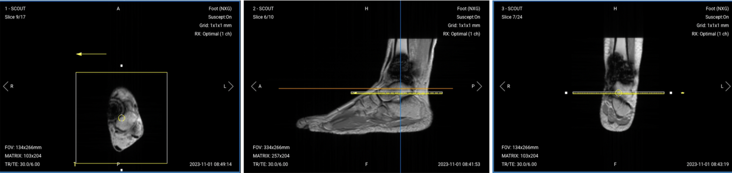
4. Capture the Initial Localizer Images
Before we can perform any MRI protocol, we must always capture initial localizer images of the patient. These images act as a guide for planning the detailed scans we will perform next.
We should always capture localizers in three planes:
Axial
Sagittal
Coronal
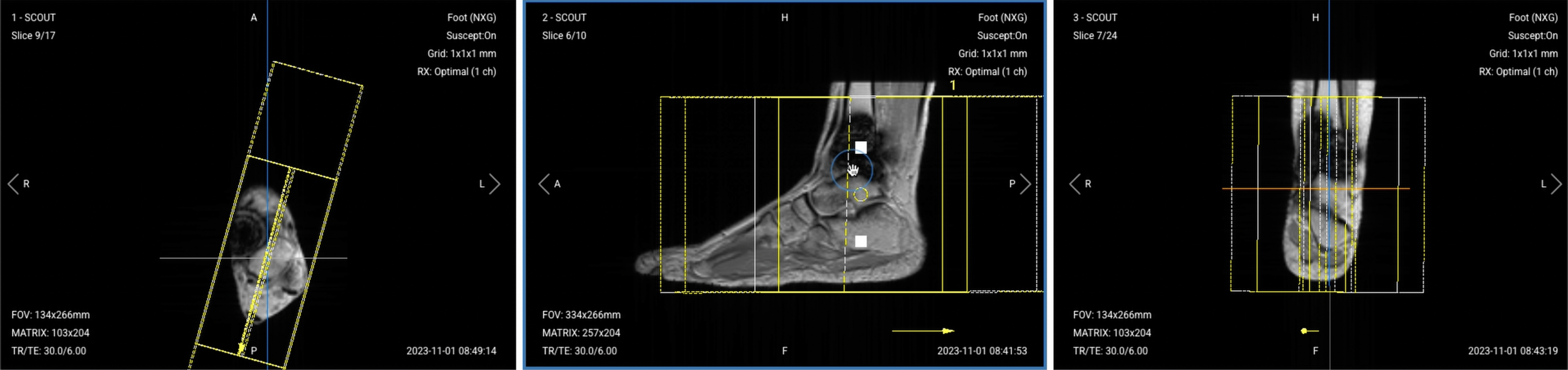
Once acquired, load the initial localizer images into the three viewports.
Then, scroll through each of the image stacks to locate a central slice that clearly shows the anatomy of the ankle.
✅ Correct Setup of Localizer Images for Ankle MRI:
Part 2: Plan and Acquire the Protocol Sequences
When all preparations are ready, we can start planning and acquiring the protocol sequences.
Let's go through the pulse sequences a standard ankle MRI protocol with metal implants includes, why we perform them, and how to set them up.
The 5 Sequences of a Standard Ankle Protocol with Metal Implants
Sagittal T1 TSE
Sagittal PD STIR
Coronal PD STIR
Axial PD STIR
Axial T2 TSE
We mainly use Turbo Spin Echo sequences with STIR fat suppression for this study. These sequences handle metal artifacts much better than gradient echo sequences and provide consistent fat suppression even near metal implants.
STIR fat suppression also works better than spectral suppression around metal, because it doesn't rely on a uniform magnetic field.
The values in the tables below are worked examples for the 1.5 T setup used in this guide. Exact numbers vary by scanner, coil and department, so treat them as a starting point rather than as fixed limits.
In the sections below, we go through how to plan and set up each sequence.
1. Sagittal T1 TSE
✅ Correct Planning:
Planning Instructions:
Use the medial and lateral malleoli as your anatomical references.
Align the slices as follows:
Axial localizer: Angle slices perpendicular to the malleoli and center over the ankle joint.
Sagittal localizer: Center the slice package over the ankle.
Coronal localizer: Ensure slices are parallel to the tibial bone.
Use appropriate geometry parameters:
Slice number: Enough slices to cover the ankle from medial to lateral (18–22 slices).
Slice thickness: 3 mm for high resolution to visualize tissues around the metal.
Slice gap: 0.3 mm (10% of slice thickness) to maintain continuity.
Set the foldover direction (phase encoding) to anterior-posterior (AP) and enable foldover suppression, because anatomy extends beyond the field of view in that direction.
Parameters for Sagittal T1 TSE:
Parameter
Recommended Values
Why These Values
Echo Time (TE)
10–15 ms
Short TE is required for T1 contrast.
Repetition Time (TR)
300–450 ms
Short TR is required for T1 contrast.
Fat Suppression
None
Bright marrow fat is what makes the interface and structural change visible here.
Field of View (FOV)
140 × 140 mm
Small FOV provides high resolution focused on ankle anatomy.
Matrix
352 × 272
352 × 272 gives 0.40 × 0.51 mm, the finest resolution here, for the tissue around the implant.
Foldover Direction (Phase)
Anterior-to-Posterior (AP)
Phase runs anterior to posterior; foldover suppression handles the aliasing this direction brings.
Number of Slices
18–22
Covers about 66 mm medial to lateral, enough for both malleoli.
Slice Thickness
3 mm
Thin enough to resolve the bone-implant interface, at a real SNR cost.
Slice Gap
0.3 mm
10% of slice thickness, which limits cross-talk without hiding anatomy.
NEX / Averages
2
To get enough SNR, while keeping scan time short.
Turbo Factor / ETL
2–4
Kept short so the effective TE stays short, preserving T1-weighting.
Bandwidth per pixel
450–550 Hz/px
High bandwidth limits metal distortion and keeps fat-water shift below one pixel at 1.5 T.
Foldover Suppression
Yes
Anatomy extends beyond the field of view anterior to posterior, the phase direction here.
Parallel Imaging
GRAPPA, acceleration factor 2
Halves the phase-encoding steps to keep scan time down, at a modest SNR cost.
2. Sagittal PD STIR TSE
✅ Correct Planning:
Planning Instructions:
Copy the slice geometry and planning from the previous Sagittal T1 TSE sequence.
Keep the same slice angulation, coverage, and positioning to ensure images of different contrasts can be clearly compared.
Parameters for Sagittal PD STIR:
Parameter
Recommended Values
Why These Values
Echo Time (TE)
40–50 ms
TE 45 ms adds mild T2 weighting, which raises the conspicuity of fluid and marrow edema.
Repetition Time (TR)
1,800–2,500 ms
Long enough for recovery between the inversion pulses, and keeps the weighting proton density rather than T1.
Fat Suppression
3 ms sinc IR pulse
Inversion recovery nulls fat without needing a uniform field, unlike spectral suppression.
Inversion Time (TI)
120–150 ms
Short TI nulls fat signal at 1.5 T to highlight inflammation and edema.
Field of View (FOV)
140 × 140 mm
Small FOV provides high resolution focused on ankle anatomy.
Matrix
352 × 272
352 × 272 gives 0.40 × 0.51 mm, the finest resolution here, for the tissue around the implant.
Foldover Direction (Phase)
Anterior-to-Posterior (AP)
Phase runs anterior to posterior; foldover suppression handles the aliasing this direction brings.
Number of Slices
18–22
Covers about 66 mm medial to lateral, enough for both malleoli.
Slice Thickness
3 mm
Thin enough to resolve the bone-implant interface, at a real SNR cost.
Slice Gap
0.3 mm
10% of slice thickness, which limits cross-talk without hiding anatomy.
NEX / Averages
3
A third average recovers SNR lost to the high bandwidth, the acceleration and the inversion pulse.
Turbo Factor / ETL
12–16
Shortens scan time, and high bandwidth and short echo spacing keep echo-train blurring acceptable.
Bandwidth per pixel
450–550 Hz/px
High bandwidth limits metal distortion and keeps fat-water shift below one pixel at 1.5 T.
Foldover Suppression
Yes
Anatomy extends beyond the field of view anterior to posterior, the phase direction here.
Parallel Imaging
GRAPPA, acceleration factor 2
Halves the phase-encoding steps to keep scan time down, at a modest SNR cost.
3. Coronal PD STIR TSE
✅ Correct Planning:
Planning Instructions:
Use the lateral and medial malleoli as your anatomical references.
Align the slices as follows:
Axial localizer: Ensure slices are parallel to the malleoli.
Sagittal localizer: Center the slice package and angle the slices parallel to the tibial bone.
Coronal localizer: Center the slice package.
Use appropriate geometry parameters:
Slice number: Cover the ankle from anterior to posterior (26–30 slices).
Slice thickness: 3 mm for consistent resolution.
Slice gap: 0.3 mm to maintain continuity.
Set the foldover direction (phase encoding) to right-left (RL) since no anatomy extends outside FOV in this direction.
Parameters for Coronal PD STIR:
Parameter
Recommended Values
Why These Values
Echo Time (TE)
40–50 ms
TE 45 ms adds mild T2 weighting, which raises the conspicuity of fluid and marrow edema.
Repetition Time (TR)
1,800–2,500 ms
Long enough for recovery between the inversion pulses, and keeps the weighting proton density rather than T1.
Fat Suppression
3 ms sinc IR pulse
Inversion recovery nulls fat without needing a uniform field, unlike spectral suppression.
Inversion Time (TI)
120–150 ms
Short TI nulls fat signal at 1.5 T to highlight inflammation and edema.
Field of View (FOV)
140 × 140 mm
Small FOV provides high resolution focused on ankle anatomy.
Matrix
352 × 256
352 × 256 gives 0.40 × 0.55 mm, fine enough to resolve the bone-implant interface.
Foldover Direction (Phase)
Right-to-Left (RL)
RL phase minimizes wraparound risk due to limited lateral anatomy.
Number of Slices
26–30
Covers about 92 mm anterior to posterior, enough for the joint and the hardware.
Slice Thickness
3 mm
Thin enough to resolve the bone-implant interface, at a real SNR cost.
Slice Gap
0.3 mm
10% of slice thickness, which limits cross-talk without hiding anatomy.
NEX / Averages
3
A third average recovers SNR lost to the high bandwidth, the acceleration and the inversion pulse.
Turbo Factor / ETL
12–16
Shortens scan time, and high bandwidth and short echo spacing keep echo-train blurring acceptable.
Bandwidth per pixel
450–550 Hz/px
High bandwidth limits metal distortion and keeps fat-water shift below one pixel at 1.5 T.
Foldover Suppression
No
No anatomy extends beyond the field of view right to left, the phase direction here.
Parallel Imaging
GRAPPA, acceleration factor 2
Halves the phase-encoding steps to keep scan time down, at a modest SNR cost.
4. Axial PD STIR TSE
✅ Correct Planning:
Planning Instructions:
Use the tibiotalar joint as your anatomical reference when it is visible. If the implant artifact obscures it, do not try to guess through the void. Angle instead from the structures you can still see, such as the tibial shaft, the talar dome margins, and the calcaneus, and cross-check against the sagittal and coronal STIR images. This is one of the reasons we acquire all three planes: when metal destroys the landmark in one plane, the other two still show it.
Align the slices as follows:
Axial localizer: Center the slice package.
Sagittal localizer: Angle slices perpendicular to the tibial shaft.
Coronal localizer: Ensure slices cover the joint space evenly.
Use appropriate geometry parameters:
Slice number: Enough to cover the ankle from superior to inferior (32–38 slices).
Slice thickness: 3 mm for high resolution.
Slice gap: 0.3 mm for continuity.
Set the foldover direction (phase encoding) to right-left (RL) to avoid wraparound.
Parameters for Axial PD STIR:
Parameter
Recommended Values
Why These Values
Echo Time (TE)
40–50 ms
TE 45 ms adds mild T2 weighting, which raises the conspicuity of fluid and marrow edema.
Repetition Time (TR)
1,800–2,500 ms
Long enough for recovery between the inversion pulses, and keeps the weighting proton density rather than T1.
Fat Suppression
3 ms sinc IR pulse
Inversion recovery nulls fat without needing a uniform field, unlike spectral suppression.
Inversion Time (TI)
120–150 ms
Short TI nulls fat signal at 1.5 T to highlight inflammation and edema.
Field of View (FOV)
140 × 140 mm
Small FOV provides high resolution focused on ankle anatomy.
Matrix
352 × 256
352 × 256 gives 0.40 × 0.55 mm, fine enough to resolve the bone-implant interface.
Foldover Direction (Phase)
Right-to-Left (RL)
RL phase minimizes wraparound risk due to limited lateral anatomy.
Number of Slices
32–38
Covers about 115 mm superior to inferior, from the distal tibia through the hindfoot.
Slice Thickness
3 mm
Thin enough to resolve the bone-implant interface, at a real SNR cost.
Slice Gap
0.3 mm
10% of slice thickness, which limits cross-talk without hiding anatomy.
NEX / Averages
3
A third average recovers SNR lost to the high bandwidth, the acceleration and the inversion pulse.
Turbo Factor / ETL
12–16
Shortens scan time, and high bandwidth and short echo spacing keep echo-train blurring acceptable.
Bandwidth per pixel
450–550 Hz/px
High bandwidth limits metal distortion and keeps fat-water shift below one pixel at 1.5 T.
Foldover Suppression
No
No anatomy extends beyond the field of view right to left, the phase direction here.
Parallel Imaging
GRAPPA, acceleration factor 2
Halves the phase-encoding steps to keep scan time down, at a modest SNR cost.
5. Axial T2 TSE
✅ Correct Planning:
Geometry copied from the Axial PD STIR sequence, so the planning view is identical.
Planning Instructions:
Copy the slice geometry and planning from the previous Axial PD STIR sequence.
Keep the same slice angulation, coverage, and positioning to ensure images of different contrasts can be clearly compared.
Parameters for Axial T2 TSE:
Parameter
Recommended Values
Why These Values
Echo Time (TE)
80–100 ms
Long TE is required for T2 contrast.
Repetition Time (TR)
1,800–3,000 ms
Long TR is required for T2 contrast.
Fat Suppression
None
Bright marrow fat is what makes the interface and structural change visible here.
Field of View (FOV)
140 × 140 mm
Small FOV provides high resolution focused on ankle anatomy.
Matrix
352 × 256
352 × 256 gives 0.40 × 0.55 mm, fine enough to resolve the bone-implant interface.
Foldover Direction (Phase)
Right-to-Left (RL)
RL phase minimizes wraparound risk due to limited lateral anatomy.
Number of Slices
32–38
Covers about 115 mm superior to inferior, from the distal tibia through the hindfoot.
Slice Thickness
3 mm
Thin enough to resolve the bone-implant interface, at a real SNR cost.
Slice Gap
0.3 mm
10% of slice thickness, which limits cross-talk without hiding anatomy.
NEX / Averages
2
To get enough SNR, while keeping scan time short.
Turbo Factor / ETL
16–20
Higher turbo factor reduces scan time, and long effective TE provides T2 weighting.
Bandwidth per pixel
450–550 Hz/px
High bandwidth limits metal distortion and keeps fat-water shift below one pixel at 1.5 T.
Foldover Suppression
No
No anatomy extends beyond the field of view right to left, the phase direction here.
Parallel Imaging
GRAPPA, acceleration factor 2
Halves the phase-encoding steps to keep scan time down, at a modest SNR cost.
How to Avoid Artifacts When Planning the Sequences
The table below lists the 5 common ankle artifacts when imaging with metal implants, and what techniques you can use to avoid them:
Artifacts
Solution – How to Avoid It
Metal artifacts
Bandwidth 488 Hz/px, 0.40 × 0.55 mm in-plane, 3 mm slices, TSE rather than gradient echo.
Chemical shift artifacts
At 488 Hz/px the fat-water shift is under half a pixel at 1.5 T.
Wrap-around artifacts
AP phase with foldover suppression on the sagittal sequences; RL phase without it on the coronal and axial.
Motion artifacts
Keep each acquisition near the 2 to 4 minutes these settings deliver.
Flow artifacts
Set the phase direction so ghosting does not cross the bone-implant interface.
Part 3: Review the Images
Finally, we will review the images to ensure all the anatomical information we need is clear.
These key structures must be clearly visible in an ankle MRI with metal implants:
Bone-implant interface
Surrounding bone marrow
Ligaments and tendons (if not obscured by metal)
Joint spaces and cartilage
Soft tissues around the implant
Signs of fluid collection or inflammation
Below, we will go through all the different image contrasts and explain their specific role in imaging the ankle with metal implants.
T1 TSE – Highlight Bone and Structural Changes
T1-weighted imaging makes fat appear bright and fluid dark. This contrast is ideal for fat-rich tissues and structural abnormalities. T1 shows anatomical structures clearly, since it helps us see where different solid tissues like muscle and fat meet.
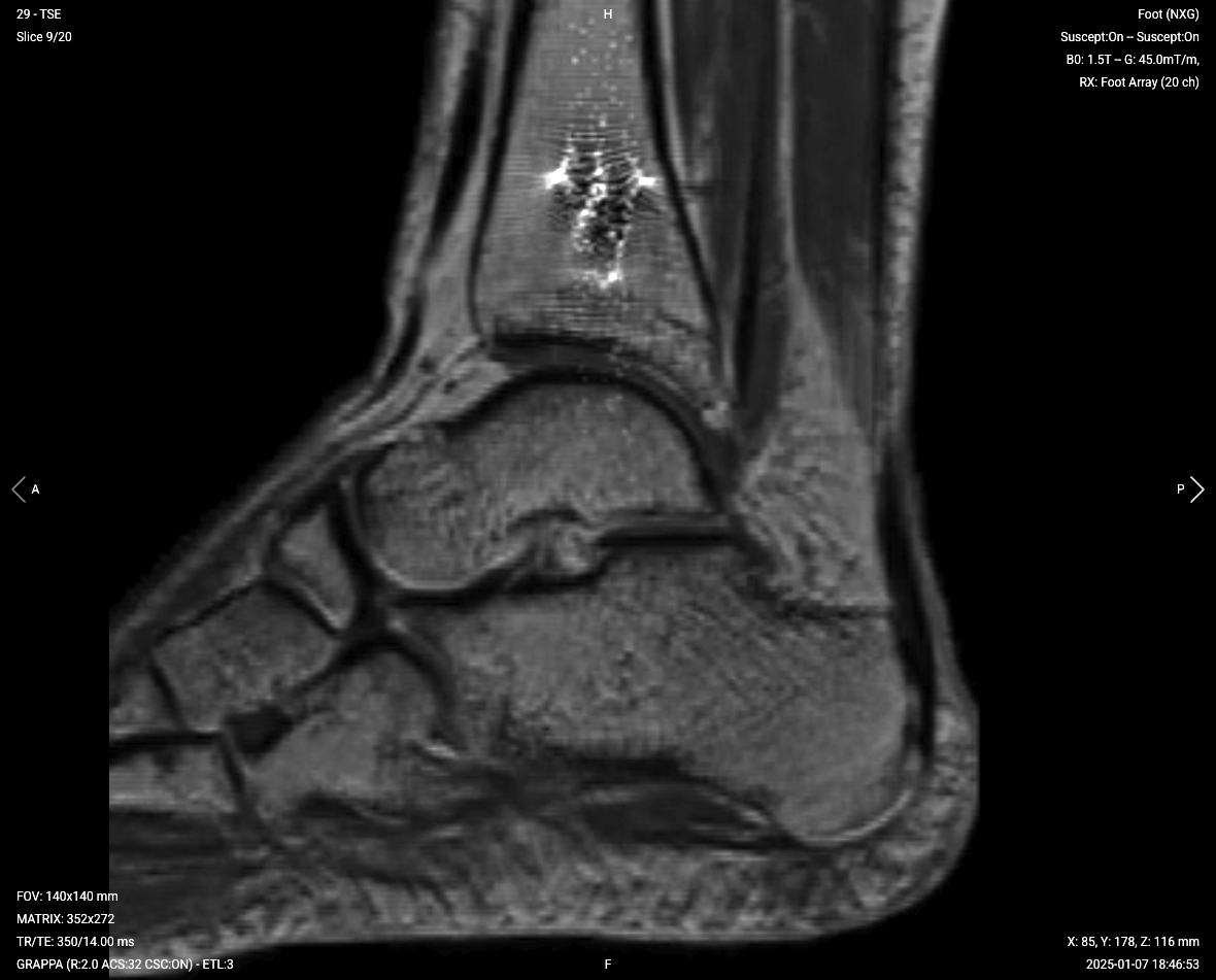
In ankle MRI with metal implants, T1 sequences are key for evaluating the bone-implant interface, detecting loosening, and assessing for avascular necrosis. The bright fat signal makes it easy to see where normal marrow has been replaced, and it is where the low-signal fracture line or necrotic margin shows up.
We capture the sagittal view to assess the ankle from a lateral perspective. This helps evaluate the tibiotalar joint and surrounding structures along the length of the ankle.
✅ Sagittal T1 TSE – Correct Image Example:
Things to Look for in Sagittal T1:
Clear visualization of bone-implant interface
Normal bright marrow signal away from metal
Loss of the normal bright marrow signal, which can indicate edema, infection, or loosening
Structural integrity of surrounding bone
PD STIR – Clearest View of Inflammation and Fluid
STIR (Short Tau Inversion Recovery) uses an inversion pulse timed to null fat signal, which makes water-rich tissue stand out clearly, even more clearly than on T2. Because it works on T1 rather than on frequency, it nulls any tissue with a T1 close to fat, which is why STIR is not used after gadolinium.
This makes STIR well suited to detecting subtle fluid-related issues, such as edema, inflammation, and infections where increased water content would otherwise be obscured by fat.
In ankle MRI with metal implants, STIR is important for identifying infections, bone marrow edema, and soft tissue inflammation. Unlike spectral fat suppression, STIR works reliably near metal because it doesn't depend on a uniform magnetic field.
We capture sagittal, coronal, and axial views to thoroughly evaluate all aspects of the ankle. Each plane provides unique information about different anatomical structures and pathology.
✅ Sagittal PD STIR – Correct Image Example:
Things to Look for in Sagittal PD STIR:
Bright signal indicating marrow edema or infection
Fluid collections around the implant
Soft tissue inflammation or abscess formation
Integrity of tendons and ligaments
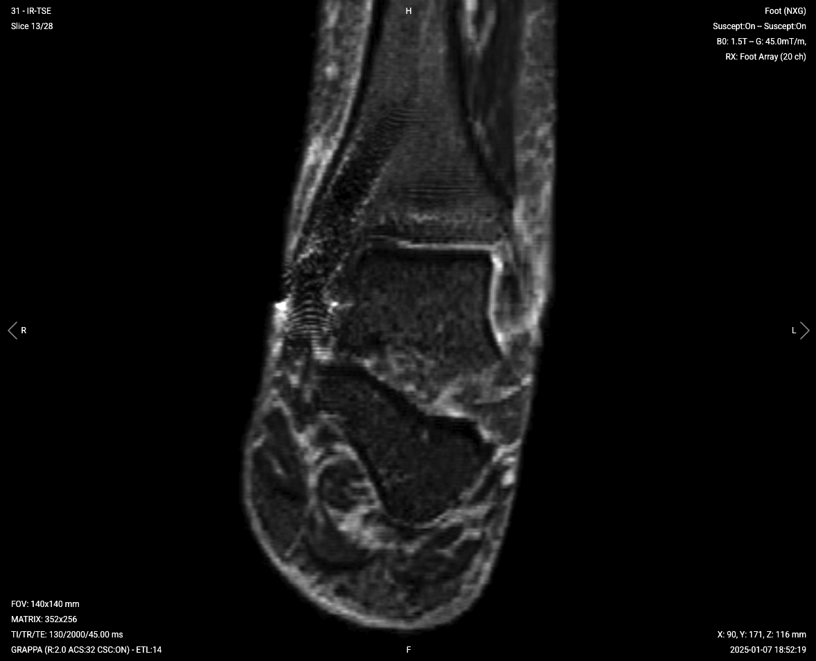
✅ Coronal PD STIR – Correct Image Example:
Things to Look for in Coronal PD STIR:
Symmetric assessment of both malleoli
Fluid in joint spaces
Bone marrow edema patterns
Soft tissue swelling or inflammation
✅ Axial PD STIR – Correct Image Example:
Things to Look for in Axial PD STIR:
Cross-sectional view of implant position
Circumferential fluid collections
Soft tissue inflammation patterns
Tendon and ligament abnormalities
T2 TSE – Highlight Fluid and Soft Tissue Detail
T2-weighted imaging makes fluids appear bright. This contrast is ideal for tissues and abnormalities with high water content.
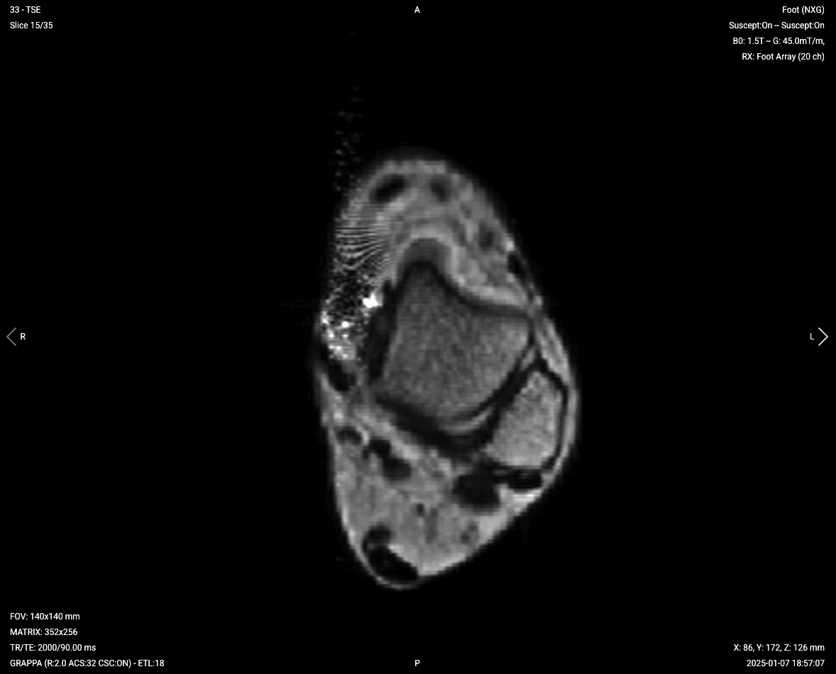
In ankle MRI with metal implants, T2 sequences help assess joint effusions, tendon tears, and ligament injuries. The bright fluid signal makes it easy to identify abnormal fluid collections that might indicate complications.
✅ Axial T2 TSE – Correct Image Example:
Things to Look for in Axial T2:
Joint effusions appearing bright
Tendon integrity and signal
Ligament tears or thickening
Cystic changes or fluid collections
Final Checks:
Before finishing an ankle MRI with metal implants, always check these 5 points to ensure diagnostic quality:
Metal Artifact Management: Ensure metal artifacts are minimized enough to visualize important structures around the implant.
Bone-Implant Interface: The interface must be visible to assess for loosening or osteolysis.
Fluid Detection: STIR sequences must clearly show any abnormal fluid collections or marrow edema.
Soft Tissue Coverage: All sequences must adequately cover tendons, ligaments, and muscles around the ankle.
Image Quality: Images must have adequate SNR despite high bandwidth settings, with minimal motion or wraparound artifacts.
Bonus: Why We Use Turbo Spin Echo With STIR Fat Suppression Around Metal
When scanning ankles with metal implants, not all sequence types handle artifacts equally well.
To understand why turbo spin echo (TSE) with STIR fat suppression is preferred, it helps to compare it directly to two common alternatives.
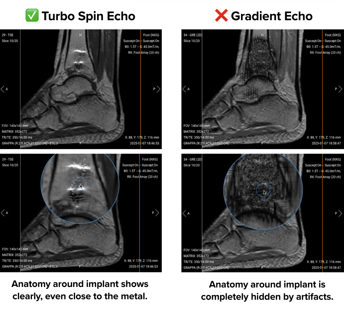
Test 1 – Turbo Spin Echo vs Gradient Echo
If you keep the same scan parameters (TR, TE, matrix, bandwidth, and geometry) and simply change the sequence type from turbo spin echo to gradient echo, the image quality changes significantly.
Turbo spin echo will typically show the ankle anatomy clearly, even close to the implant. The metal artifact is still present, but the structures around it are usually well-defined.
With gradient echo, however, the image near the metal often becomes unreadable. The artifact appears larger and more intense, and nearby anatomy may be completely obscured.
This happens because the refocusing pulses in turbo spin echo recover much of the signal lost to reversible dephasing around metal, which makes it far less sensitive to susceptibility than gradient echo. Geometric distortion is not corrected by refocusing, which is why high bandwidth and small voxels still matter.
Gradient echo, however, lacks these pulses, so the artifacts appear stronger and cover more of the image.
One parameter cannot be matched. The gradient echo comparison uses a 25° excitation flip angle, whereas turbo spin echo uses 90° excitation with 180° refocusing pulses. That difference is the point of the test rather than a flaw in it, because those refocusing pulses are exactly what gradient echo lacks.
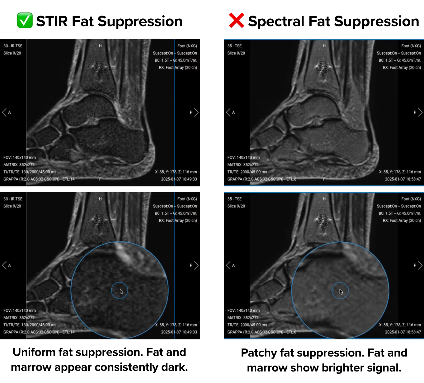
Test 2 – STIR vs Spectral Fat Suppression
Now consider a sagittal PD sequence with the same geometry, TE, TR, bandwidth per pixel, and acceleration, where the fat suppression method changes from STIR to spectral.
One parameter is not matched here. The spectral acquisition uses a turbo factor of 8 against 14 on the STIR image, so it is slightly sharper. SNR is the same on both. That works against the point being made rather than for it: the spectral image is the sharper of the two and still shows uneven fat suppression near the implant.
With STIR, fat suppression remains even across the field of view. Bone marrow shows a uniform low signal, and subcutaneous fat appears consistently dark.
But with spectral fat suppression, the fat suppression may appear patchy. You might see bright signals remaining in bone marrow and subcutaneous fat, especially near the implant.
This difference is due to how the sequences work.
Spectral fat suppression works by identifying fat based on its frequency. It requires a uniform magnetic field to apply the suppression accurately. But metal implants disrupt that uniformity, which causes the technique to fail in some regions.
STIR works differently. It uses timing (inversion recovery) to suppress fat, not frequency. This allows STIR to perform more reliably in areas with magnetic field distortion, such as around metal implants.
This is why ankle MRI protocols with implants typically use TSE pulse sequences with STIR for fat suppression.
Turbo spin echo handles metal distortion better than gradient echo.
STIR fat suppression performs more reliably near metal than spectral fat suppression.
This combination helps reduce artifacts, improves visualization of soft tissues, and enables better diagnostic quality around implants.

.svg)