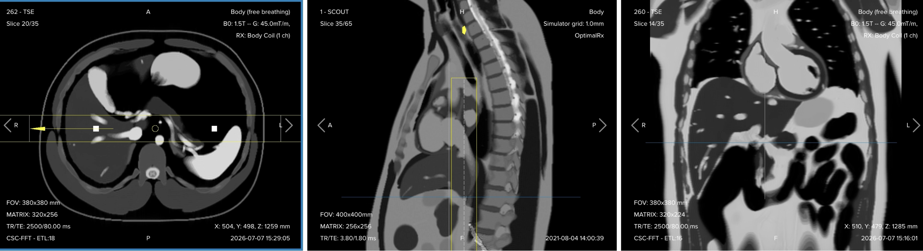
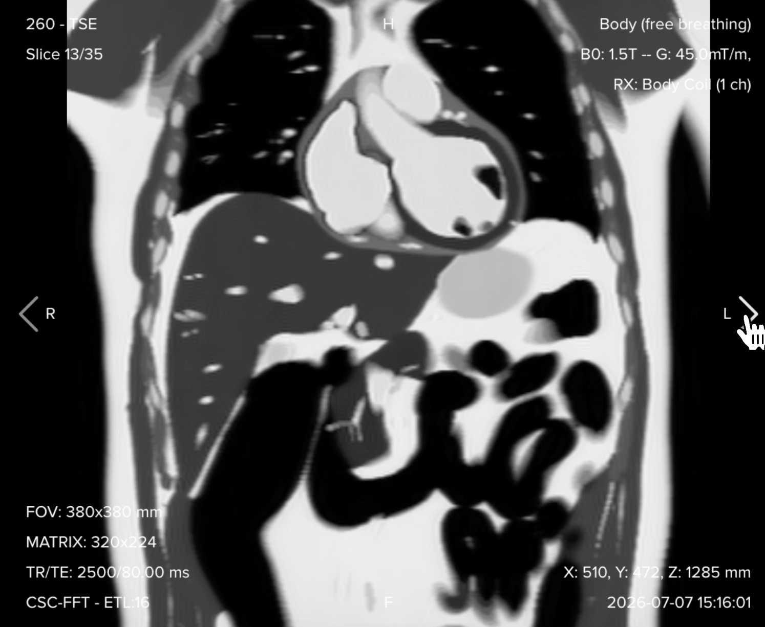
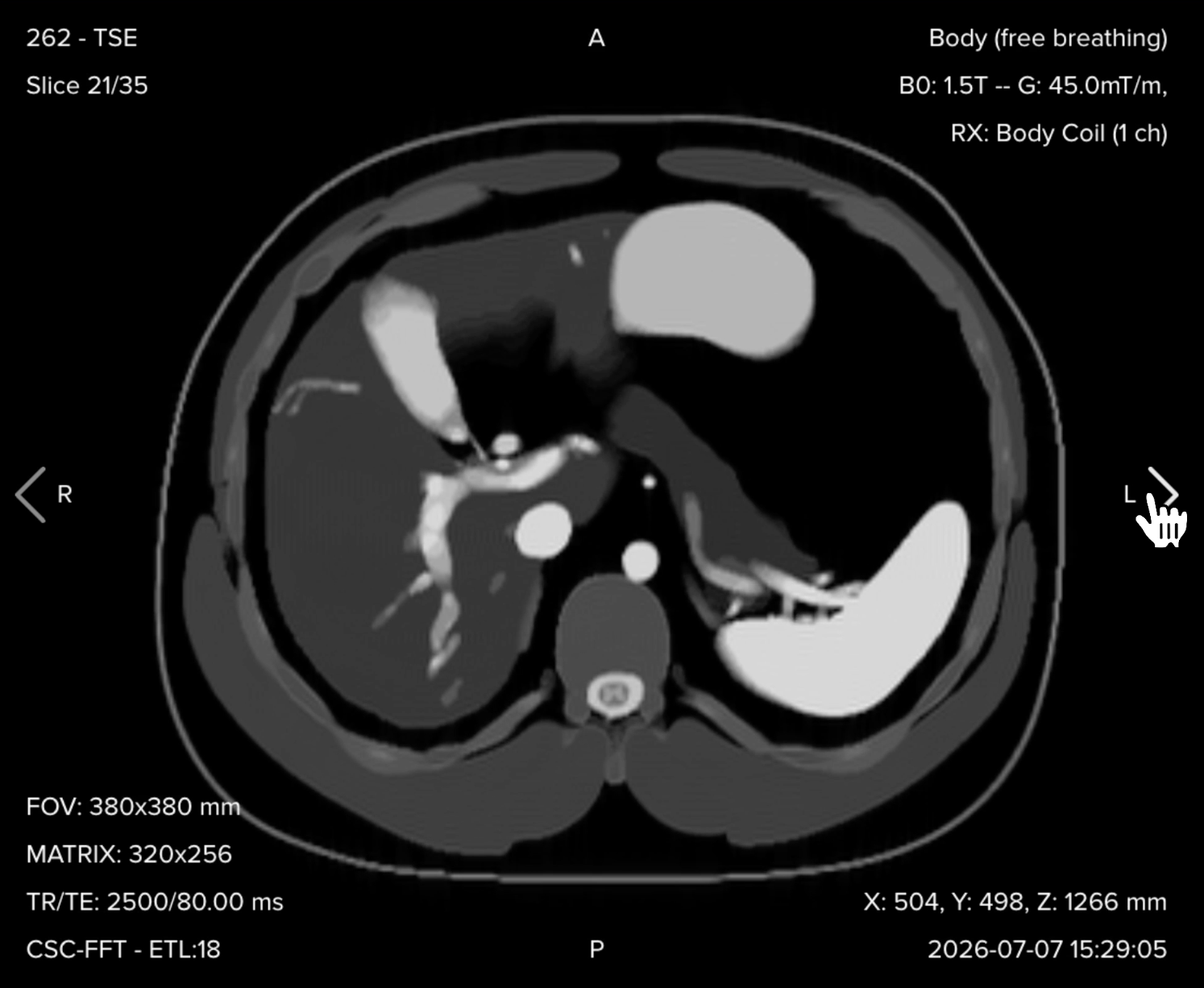
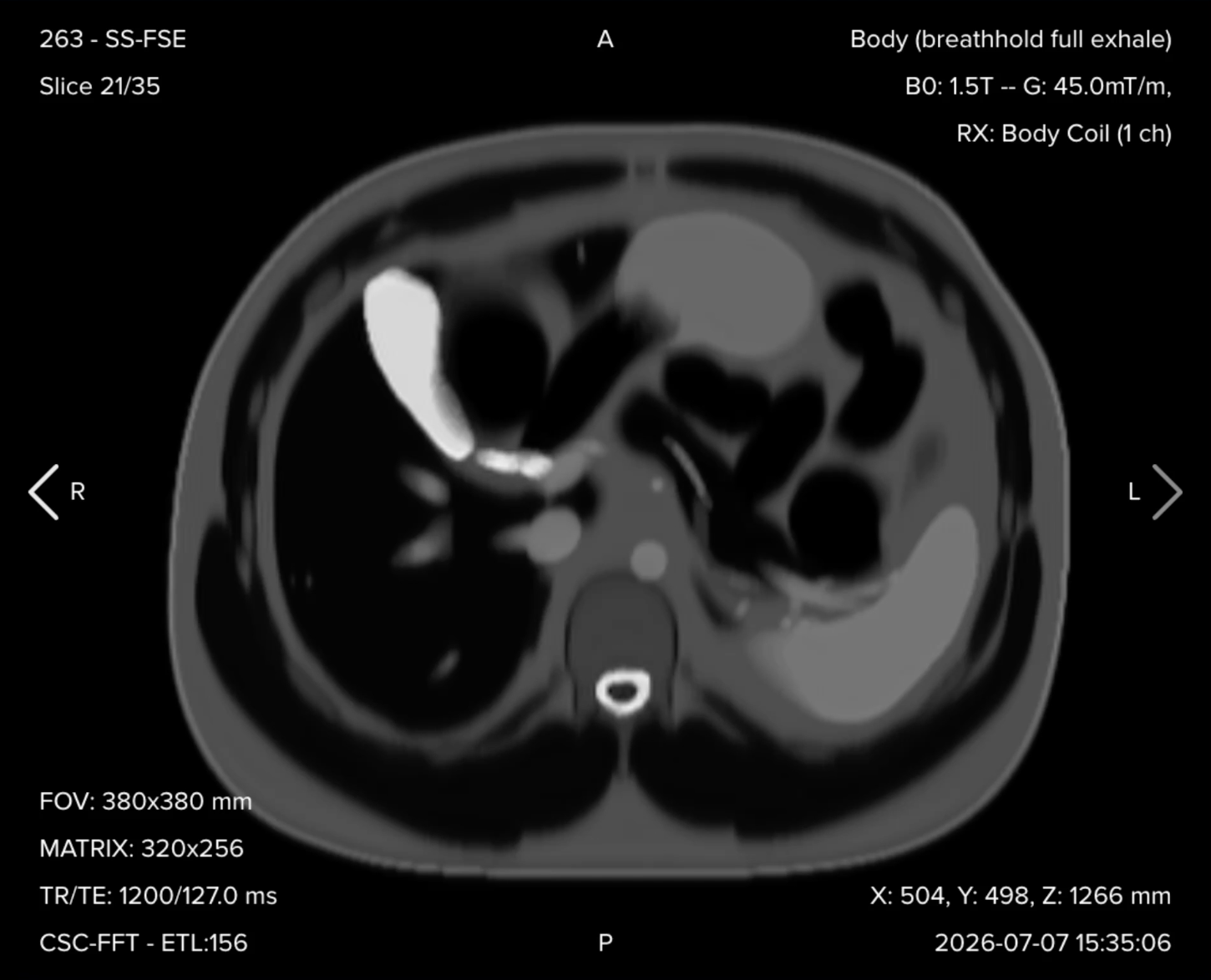
This step-by-step guide is for MRI students, radiographers, and technologists who wish to improve their planning skills and master the MRCP protocol.
What you will learn:
Key factors in MRCP, including trade-offs.
Patient and scanner setup tips.
Best pulse sequences and planning techniques.
Ways to avoid common artifacts.
What great MRCP images should look like.
Key Takeaways
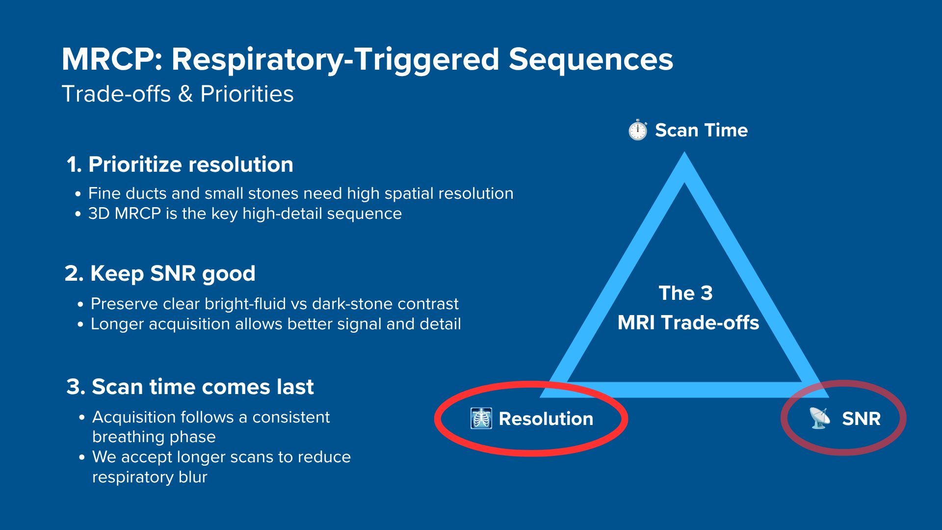
We use two sequence groups, with two opposite priorities: resolution and SNR generally come first in one, scan time in the other. But neither works until motion is controlled.
Respiratory-triggered sequences, like the 3D MRCP, spend time to keep resolution and SNR high, since the ducts are tiny fluid-filled tubes that need both to stay visible. Breath-hold sequences, like the single-shot and radial, spend detail to keep scan time short instead, since the upper abdomen moves constantly with breathing and respiratory motion is the biggest practical threat to image quality.
The 3D MRCP is the sequence the diagnosis rests on.
Its thin near-isotropic voxels map the duct tree and reconstruct in any plane, so it carries the fine duct detail. The other five sequences supply anatomical context, inflammation contrast, tissue characterization, and a fast motion-resistant backup for when the 3D acquisition is degraded.
Avoid these 5 common MRCP artifacts.
Artifact
Solution – How to Avoid It
Respiratory motion
Coach the patient on calm, regular breathing before the scan, and use respiratory or navigator-triggered 3D MRCP when available. If the 3D sequence is degraded, fall back on the fast 2D thick-slab MRCP as a motion-resistant backup.
Susceptibility (gas, clips, pneumobilia)
Cross-check any dark focus against the single-shot and 3D MRCP source images. Check for pneumobilia, clips, stents, or prior sphincterotomy before calling it a stone.
Review the finding across multiple planes and on the source images; a true stone stays within the duct on every slice. A pulsation artifact lines up with an adjacent vessel, most often the right hepatic artery at the common hepatic duct or the gastroduodenal artery at the mid CBD.
Partial volume / MIP averaging
Never rely on the thick MIP image alone. Always review the thin 3D source images, since MIP reconstruction can hide small stones or exaggerate strictures and blur.
GI fluid overlap
Fast beforehand. Use a site-approved negative oral contrast agent when local protocol allows it, such as pineapple juice, to darken bright stomach and duodenal fluid that can overlap the bile duct.
Intro to the MRCP Protocol
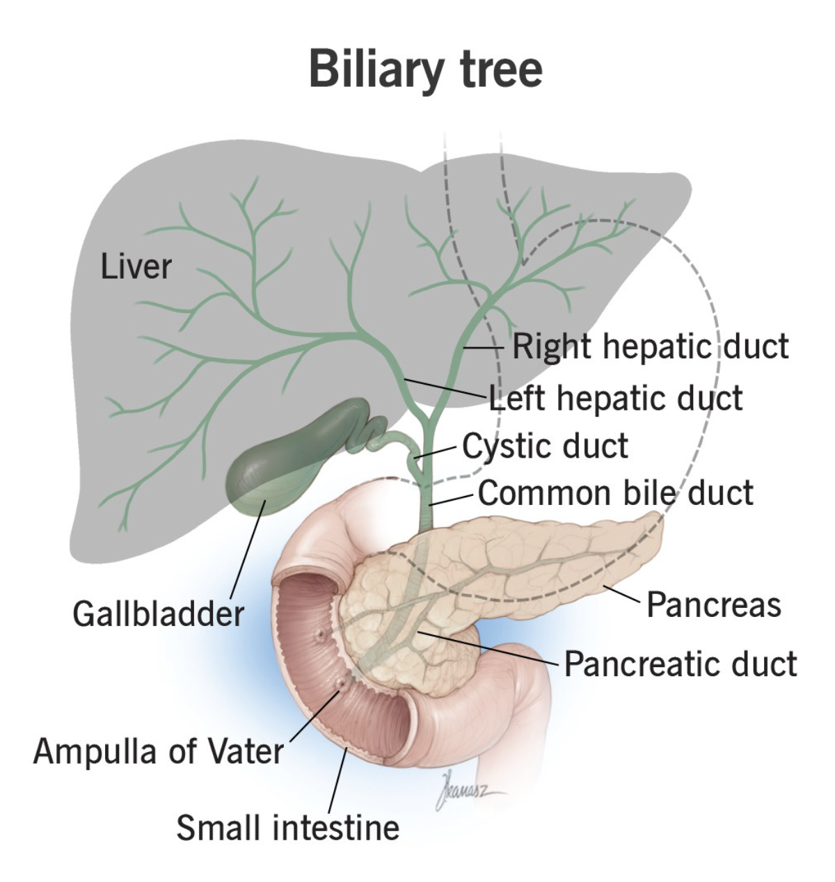
MRCP, or magnetic resonance cholangiopancreatography, evaluates the biliary and pancreatic duct systems using heavily T2-weighted imaging. This makes static fluids like bile and pancreatic juice appear bright, without invasive procedures or ionizing radiation. Stones contain no free fluid, so they appear as dark filling defects against that bright background.
The protocol combines routine upper-abdominal sequences with dedicated MRCP acquisitions, so we assess both the abdominal organs and the fine duct anatomy in one study.
After liver tests and abdominal ultrasound, MRCP is a first-line non-invasive test for suspected common bile duct stones and biliary obstruction, alongside endoscopic ultrasound.
In MRI, we always face a trade-off between 3 key metrics:
Scan Time: How fast a pulse sequence can be completed.
Resolution: How much detail the image can display.
SNR: How clear the image is, meaning how much signal we have compared with noise.
Improving one of these metrics often reduces the performance of the others. To decide what trade-offs to make, we must consider the needs of each clinical situation.
For MRCP, we face three specific challenges:
Tiny structures. The main pancreatic duct is usually only a few millimeters wide, with published reference values of roughly 3 mm below age 65 and 4 mm from age 65, and stones or strictures can be smaller still. Without high spatial resolution, partial volume averaging blurs them together and small findings vanish.
Fluid-based contrast. The duct signal comes mainly from fluid. Heavily T2-weighted imaging keeps static bile and pancreatic juice bright against a darker background, so we need enough SNR to hold the bright-fluid to dark-stone distinction clear. That gets SNR-sensitive when voxels are small and echo times are long.
Constant motion. The upper abdomen moves with breathing and bowel motion, and the high-detail scan takes minutes.
Therefore, we typically:
Prioritize resolution because the fine duct detail is the diagnosis, and
Keep SNR high enough for clarity.
But neither matters until motion is controlled, and one scan usually cannot maximize resolution, SNR, and speed at once.
So the protocol takes a two-pronged approach, splitting its sequences into two groups: one optimized for detail, one for speed.
1. The respiratory-triggered sequence group: scan time comes last
These sequences acquire data during a consistent part of the breathing cycle, usually near end-expiration, which reduces motion rather than freezing it, at the cost of minutes.
Scan time is what all three sequences in this group spend last, but what they spend it on differs: the 3D MRCP spends it on resolution, while the coronal T2 and axial T2 fat-sat spend it on coverage and inflammation contrast instead.
The 3D MRCP is the most important sequence. Its thin near-isotropic voxels, roughly 1.4 mm in-plane by 1.6 mm slice, resolve small stones and fine ducts and reconstruct in any plane, and its volumetric readout supplies the SNR those thin slices spend. The coronal and fat-suppressed T2 images ride along in the same group, trading time for clean, detailed anatomy.
2. The breath-hold sequence group: 1) scan time, 2) SNR, 3) resolution
These sequences finish inside a single breath-hold or a single shot, so respiratory motion has little chance to blur them, though bowel motion or a failed breath-hold still can.
Speed comes first, and detail is what gets sacrificed. The thick slab collapses through-plane detail into one projection, and single-shot readouts come out softer than the triggered images. This group keeps the study diagnostic when the patient cannot hold still or breathe regularly.
Strategy and Priority for Each MRCP Sequence
This table shows a breakdown of every sequence in standard MRCP protocol, the motion-control strategy we use, and what to prioritize in acquisition.
Note! Prioritizing resolution in MRCP is only a general guideline, NOT a strict rule. If your patient cannot breathe regularly or hold still, the fastest diagnostic image beats the sharpest non-diagnostic one. The right balance always depends on the needs of your patient and clinic.
Note on Other MRCP Variants
Grouping and triggering differ by vendor and site, so a sequence that is respiratory-triggered here may be run breath-hold elsewhere.
Some centers use breath-hold 3D MRCP with compressed sensing to bring near-3D duct detail into one breath-hold, though heavy acceleration can reduce small-duct visibility.
Secretin MRCP changes the trade-off further, adding repeated timed thick-slab images after IV secretin to assess pancreatic duct filling and function, where temporal timing outranks spatial resolution. These are not the sequences demonstrated in this video.
MRCP Health Conditions and the MRI Sequences That Reveal Them
The MRCP study can help us diagnose a wide range of health conditions. The table below lists some of the most common conditions and what pulse sequences reveal them:
Common conditions
Clearly seen on sequence
Why this sequence?
• Rough level of biliary obstruction
• Large extra-biliary masses
Cor T2
A multi-shot T2 TSE covering the whole upper abdomen along the axis of the biliary tree. Good for orientation and catching large findings, though the exact obstruction level and fine duct detail are confirmed on 3D MRCP.
Fat suppression removes bright background fat and the multi-shot readout adds resolution, so inflammatory fluid, wall thickening, and edema show up where a faster sequence would blur them.
• Possible CBD stones as dark filling defects
• Biliary dilatation
Ax T2 SS-TSE
Freezes a slice in about one second, resisting motion, which is its main strength. This makes it the go-to quick duct screen when breath-holding is poor, though flow artifact can mimic a filling defect, so suspected stones are confirmed on 3D MRCP source images.
Separates fat and water signal into four image sets, telling fat or blood apart from a true lesion. Useful for an iron or susceptibility clue too, though formal iron quantification needs a dedicated multi-echo method. Not the main sequence for finding stones.
• CBD stones and biliary obstruction
• Strictures: PSC or cholangiocarcinoma pattern
• Duct variants and IPMN communication
3D MRCP
The main duct-map sequence. Ultra-long echo times leave mostly static fluid visible, and thin near-isotropic voxels reconstruct the duct system in any plane. A stricture here shows the narrowing pattern, not full tumor staging, which needs contrast T1, DWI, or CT/EUS. Very small stones can still be missed, so source images are always checked alongside the MIP.
• CBD stones and biliary obstruction
• Ductal dilatation
Radial SS-TSE FS
Each thick slab gives a motion-resistant projection image in about one to two seconds, so it's the backup when 3D MRCP is degraded by motion. It shows the same duct pathology as the 3D, just faster and coarser.
How to Perform an MRCP
The step-by-step guide below will show you how to set up and perform an MRCP protocol in practice.
We will perform the protocol in 3 parts:
Set up the Patient and MRI Scanner
Plan and Acquire the Protocol Sequences
Review the Images
Part 1: Set up the Patient and MRI Scanner
1. Prepare the Patient
MRCP is one of the few protocols where preparation before the patient reaches the table directly affects image quality.
Fasting: Ask the patient to fast for 4–6 hours when the clinical situation allows. This reduces bright fluid in the stomach and duodenum, and lets the gallbladder distend.
Negative oral contrast (optional, site-dependent): Bright gastric and duodenal fluid can sit on top of the common bile duct and hide it. Purpose-built agents such as ferumoxsil were once used for this but have since been withdrawn from the market, which is a large part of why many departments now use pineapple juice instead. It works because its manganese content shortens the T2 of the fluid it mixes with, so at MRCP’s very long echo times that fluid loses nearly all signal. No official body recommends a specific volume. Published studies have used 150–400 mL, given 15–30 minutes before scanning, and the amount needed depends on the manganese concentration of the specific juice, so follow a locally validated protocol.
Breathing coaching: Practice breath-hold instructions before the patient enters the bore, and test both exhale and inhale. Many patients hold their breath far more reliably one way, and picking the better one keeps slice positions consistent between sequences.
2. Position the Patient in the Scanner
Lay the patient supine with the upper abdomen centered at the scanner’s isocenter.
Use an anterior body array coil on top of the upper abdomen, combined with the posterior spine coil integrated into the scanner table. This gives full signal coverage of the liver, gallbladder, biliary tree, and pancreas.
Arms can be positioned above the head or alongside the body. If they rest alongside the body they sit near the field of view in the right-to-left direction, which is why foldover suppression matters on the coronal sequences.
Once the patient is in place, review your scanner’s hardware settings.
In this guide, we will use the following settings:
Scanner Setting
Value
Why This Value
Magnetic field strength
1.5 T
The most common clinical field strength, giving enough SNR for this protocol with less susceptibility and B1 artifact than 3 T, and fewer dielectric artifacts in the abdomen.
Maximum gradient strength
45 mT/m
Provides strong, versatile gradient performance that supports fast imaging and precise spatial encoding.
Receive coil
Anterior body array + posterior spine coil
Full anterior-to-posterior coverage of the upper abdomen with strong signal reception.
This hardware setup is widely used in clinical practice. It balances acquisition time, image quality, and patient comfort.
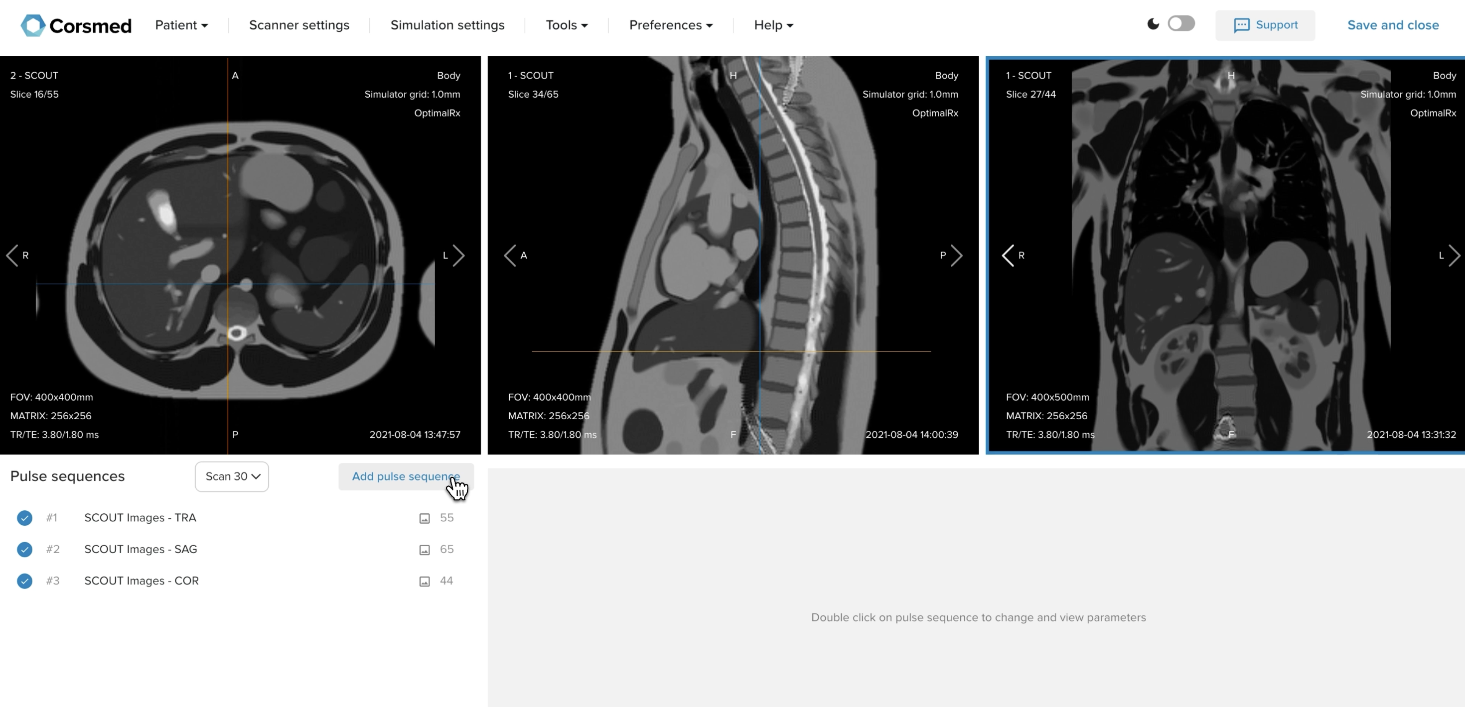
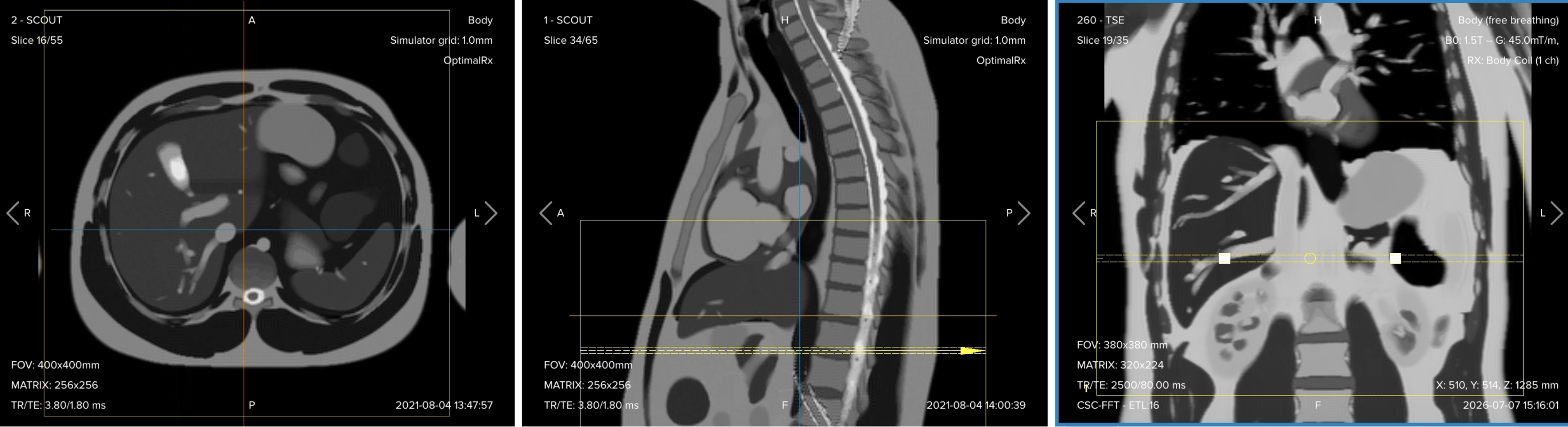
4. Capture the Initial Localizer Images
Every MRI protocol starts with localizer images of the patient. These images act as a guide for planning the detailed scans we will perform next.
Select the abdominal region, save it, and run the localizers.
We should always capture localizers in three planes:
Axial
Sagittal
Coronal
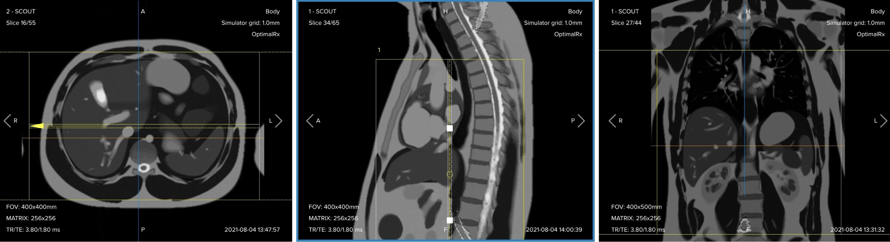
Once acquired, load the localizer images into the three viewports. Then scroll through each stack to locate a central slice that clearly shows the anatomy of the upper abdomen.
✅ Correct Setup of Localizer Images for MRCP:
Part 2: Plan and Acquire the Protocol Sequences
When all preparations are ready, we can start planning and acquiring the protocol sequences.
Let’s go through the pulse sequences a standard MRCP protocol includes, why we perform them, and how to set them up.
The 6 Sequences of a Standard MRCP Protocol
Coronal T2 TSE
Axial T2 FS TSE
Axial T2 SS-TSE
Axial GRE Dixon
3D MRCP
Radial SS-TSE FS
Sequences 1, 2, and 5 belong to the respiratory-triggered group. Sequences 3, 4, and 6 belong to the breath-hold group.
Note! Your facility may have its own local policies, so the protocol might differ in some of these sequences. If they differ, then always follow your own institution's guidelines.
In the sections below, we go through how to plan and set up each sequence.
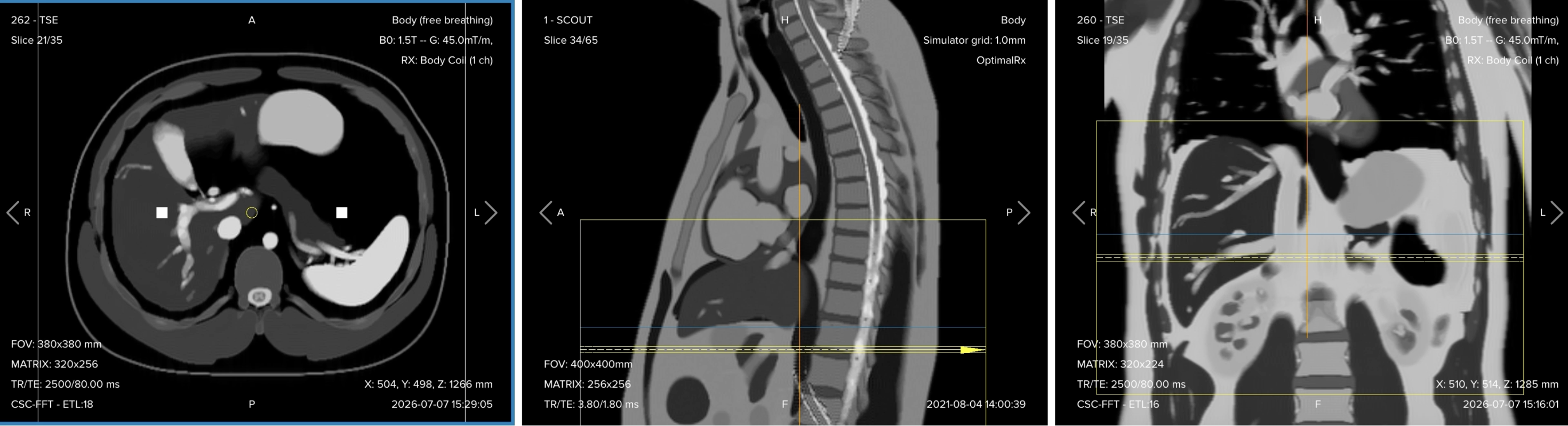
1. Planning Coronal T2 TSE
✅ Correct Planning:
Planning Instructions:
Plan in the true coronal plane, covering the entire hepatobiliary system.
Use appropriate geometry parameters:
Coverage: From the anterior abdominal wall back to the kidneys, including liver, gallbladder, pancreas, spleen, and upper kidneys.
Slice number: 32–38, enough for that anterior-to-posterior block.
Slice thickness: 6 mm, thick enough to keep SNR up across the coverage while still resolving duct anatomy.
Slice gap: 1 mm, which is 17% of the slice thickness and limits cross-talk without hiding anatomy.
Set the foldover direction (phase encoding) to right-to-left (RL) and activate foldover suppression, so the arms and body wall do not alias into the image.
Acquire with respiratory triggering. This is a multi-shot TSE that takes a few minutes, so it follows the breathing cycle rather than a breath-hold.
Tip: You can display your slices in either box view or slice view. Pick whichever helps you check coverage, angle, and position most clearly.
Parameters for Coronal T2 TSE:
Parameter
Recommended Values
Why These Values
Effective Echo Time (TE)
80–100 ms
Long TE is required for T2 contrast.
Repetition Time (TR)
2,000–2,500 ms
Long TR is required for T2 contrast. With respiratory triggering, the effective TR follows the breathing cycle.
Field of View (FOV)
380 × 380 mm
Covers the full width of the upper abdomen at this patient size.
Matrix
320 × 224
High read matrix for in-plane detail, reduced phase matrix to hold scan time down on a multi-shot readout.
Foldover Direction (Phase)
Right-to-Left (RL)
Matches the shape of the coronal upper abdomen.
Number of Slices
32–38
Enough to cover from the anterior abdominal wall back to the kidneys.
Slice Thickness
6 mm
Thick enough to keep SNR up across the whole upper abdomen, while still resolving the gallbladder and duct anatomy.
Slice Gap
1 mm
17% of slice thickness, which limits cross-talk without hiding anatomy.
NEX / Averages
1
One average is enough here, since a second would double the number of respiratory cycles the acquisition needs.
Bandwidth per pixel
225–250 Hz/px
Fat-water shift is about 224 Hz at 1.5 T, so this keeps the shift just under one pixel. Going lower would gain SNR but widen chemical shift at the organ borders.
Turbo Factor / ETL
14–18
Higher turbo factor reduces scan time, and long effective TE provides T2 weighting.
Parallel Imaging
No
Scan time is the lowest priority here, and this sequence already fits its respiratory window, so there's nothing to gain by trading SNR for it.
Partial Fourier
Phase-conjugate (half-Fourier), factor 0.6
Fills part of k-space and reconstructs the rest, shortening the acquisition without an extra averaging pass.
Foldover Suppression
Yes
Limits aliasing from the arms and body wall in the RL direction.
Breath-hold Mode
Free breathing
Multi-shot TSE takes minutes, which is far too long for a breath-hold, so it follows the respiratory cycle instead.
2. Planning Axial T2 FS TSE
✅ Correct Planning:
Planning Instructions:
Plan in the axial plane. Right-click on the axial localizer and set the in-plane position, which also sets the correct orientation under the Geometry tab.
Use appropriate geometry parameters:
Coverage: From the hepatic dome down to the kidneys.
Slice number: 32–38.
Slice thickness: 6 mm, with a 1 mm gap.
Review your slice package on top of a high-resolution image, such as the coronal T2, and scroll through to confirm the abdominal dome and kidneys are both covered.
Set the foldover direction (phase encoding) to anterior-to-posterior (AP) to limit aliasing.
Foldover suppression can stay off here, since no anatomy extends beyond the field of view in the AP direction. Leaving it off also reduces scan time.
Acquire with respiratory triggering, the same as the coronal T2.
Parameters for Axial T2 FS TSE:
Parameter
Recommended Values
Why These Values
Effective Echo Time (TE)
80–95 ms
Long TE is required for T2 contrast.
Repetition Time (TR)
2,000–2,500 ms
Long TR is required for T2 contrast and allows enough slices per acquisition.
Field of View (FOV)
380 × 380 mm
Sized to the patient's abdominal width, matching the coronal T2.
Matrix
320 × 256
Higher phase matrix than the coronal T2, resolving wall thickening and small fluid collections.
Foldover Direction (Phase)
Anterior-to-Posterior (AP)
Matches the shape of the axial abdomen, which limits wraparound.
Number of Slices
32–38
Enough to cover from the hepatic dome to the kidneys.
Slice Thickness
6 mm
Thick enough to keep SNR up from the hepatic dome to the kidneys, while still resolving gallbladder wall thickening.
Slice Gap
1 mm
17% of slice thickness, which limits cross-talk without hiding anatomy.
NEX / Averages
2
Higher than the coronal T2, since the fat suppression pulse removes signal that has to be recovered.
Bandwidth per pixel
220–250 Hz/px
Kept low to protect the SNR that the fat suppression pulse removes; chemical shift is less of a concern here since fat suppression already reduces the fat signal that would cause it.
Turbo Factor / ETL
16–20
Higher turbo factor reduces scan time, and long effective TE provides T2 weighting.
Parallel Imaging
No
Would cost SNR this fat-sat sequence is already short on, for a time saving it doesn't need.
Partial Fourier
No
Not needed here since the turbo factor and TR already keep the acquisition within its respiratory window.
Foldover Suppression
No
No anatomy extends beyond the FOV in the AP direction, and leaving it off shortens scan time.
Fat Suppression
Spectral
Removes fat signal so inflammation and edema stand out against a darker background.
Breath-hold Mode
Free breathing
Multi-shot TSE needs minutes to acquire, so it follows the respiratory cycle instead of a breath-hold.
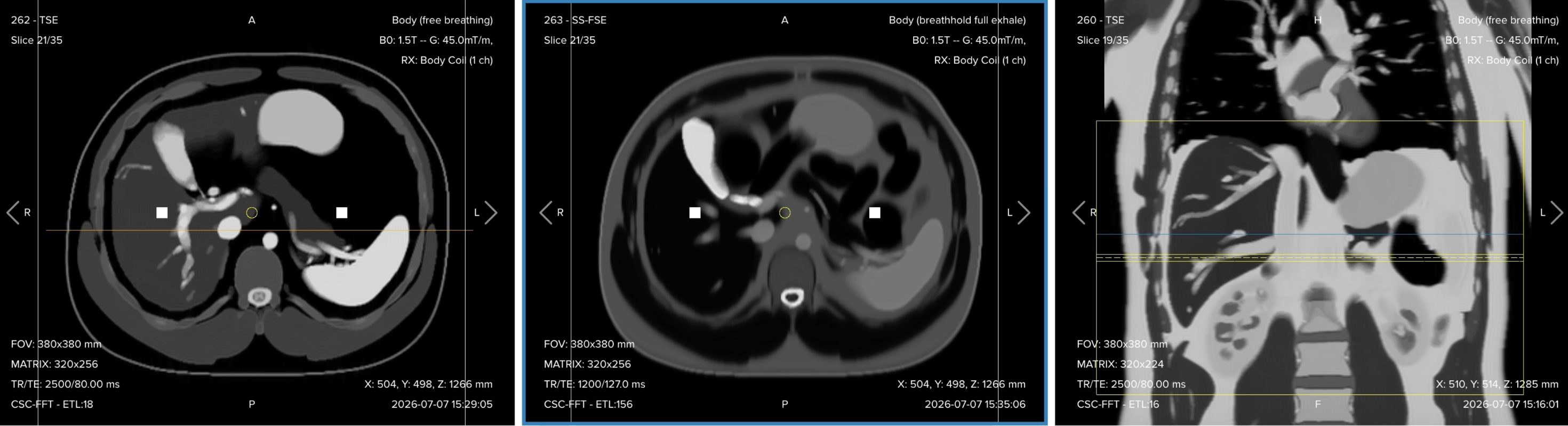
3. Planning Axial T2 SS-TSE
The SS tag stands for single-shot. This sequence captures the complete k-space for each slice in one shot, which makes it far faster than the multi-shot sequences before it.
✅ Correct Planning:
Planning Instructions:
Copy the slice geometry and planning from the previous axial T2 FS TSE sequence.
Keep the same slice angulation, coverage, and positioning so images of different contrasts can be clearly compared.
Acquire as a breath-hold, at exhale or inhale depending on which your patient performs more reliably.
Parameters for Axial T2 SS-TSE:
Parameter
Recommended Values
Why These Values
Effective Echo Time (TE)
120–140 ms
Higher TE than the axial T2 FS gives better fluid-to-soft-tissue contrast, leaning toward highlighting fluid-containing structures.
Repetition Time (TR)
1,000–1,500 ms
Each slice is a single shot, so TR sets the interval between slices rather than the contrast.
Field of View (FOV)
380 × 380 mm
Copied from the axial T2 FS for direct comparison.
Matrix
320 × 256
Copied from the axial T2 FS. The softer look comes from the single-shot readout and half-Fourier filling, not from a smaller matrix.
Foldover Direction (Phase)
Anterior-to-Posterior (AP)
Matches the axial anatomy shape.
Number of Slices
32–38
Copied from the axial T2 FS.
Slice Thickness
6 mm
Copied from the axial T2 FS.
Slice Gap
1 mm
Copied from the axial T2 FS.
NEX / Averages
1
Single average, since the point of this sequence is speed.
Bandwidth per pixel
600–700 Hz/px
Roughly three times the 224 Hz/px chemical shift threshold at 1.5 T, which shortens the readout enough to read a whole slice in one shot.
Partial Fourier
Phase-conjugate (half-Fourier), factor 0.6
Fills only part of k-space and reconstructs the rest, which is what enables the single-shot readout.
Parallel Imaging
No
Half-Fourier already supplies the acceleration this readout needs, and adding more would cost SNR.
Foldover Suppression
No
Copied from the axial T2 FS, keeps acquisition fast.
Breath-hold Mode
Exhale or inhale
Each slice freezes in roughly one second, but the full stack of 32–38 slices takes about 30–45 seconds, so it is typically split across two or three breath-holds. Pick whichever your patient holds more reliably.
4. Planning Axial GRE Dixon
✅ Correct Planning:
Planning Instructions:
Copy the slice geometry from one of your previous axial sequences using the Custom copy option.
This time, exclude the phase matrix from the copy and keep everything else. The Dixon runs at a lower phase matrix to hold each breath-hold short.
Through-plane resolution and central position stay the same, so the radiologist can compare all sequences at matching levels.
Acquire as a breath-hold.
Parameters for Axial GRE Dixon:
Parameter
Recommended Values
Why These Values
Echo Time (TE)
4.5 ms
At 1.5 T, fat and water return to the in-phase condition every 4.4 ms, so 4.5 ms lands on an in-phase echo.
Second-echo Time Difference
2.24 ms
Half a fat-water phase cycle at 1.5 T, placing the second echo at 6.74 ms, which is opposed-phase. The two echoes are what make the Dixon separation possible.
Repetition Time (TR)
150–200 ms
Paces the gradient echo readout and, together with the phase matrix, sets total scan time.
Flip Angle
15°
Gives proton-density-like contrast rather than strong T1 weighting, keeping both fat and water visible in each reconstruction.
Field of View (FOV)
380 × 380 mm
Copied from the axial T2 sequences.
Matrix
320 × 224
Reduced phase matrix compared with the axial T2 sequences, which is the resolution cost of fitting the acquisition into one breath-hold.
Foldover Direction (Phase)
Anterior-to-Posterior (AP)
Matches the axial anatomy shape.
Number of Slices
32–38
Copied from the axial T2 sequences.
Slice Thickness
6 mm
Keeps through-plane resolution equivalent to the other axials.
Slice Gap
1 mm
Copied from the axial T2 sequences.
NEX / Averages
1
Single average keeps scan time short enough for one breath-hold.
Bandwidth per pixel
600–700 Hz/px
Wide bandwidth is what allows both echoes to be read at the exact timings the Dixon method needs, and it keeps chemical shift well under a pixel.
Parallel Imaging
GRAPPA, acceleration factor 2
Halves the phase-encoding steps, bringing each breath-hold to roughly 17 seconds.
Partial Fourier
No
Not needed once GRAPPA already brings each breath-hold to a comfortable length.
Foldover Suppression
No
No anatomy extends beyond the FOV in the AP direction.
Fat Suppression
None (reconstructed)
Fat and water are separated mathematically from the two echoes, not by a suppression pulse.
Breath-hold Mode
Exhale or inhale
Acquired across three short breath-holds of roughly 15–20 seconds each. Match the direction used on the single-shot to keep slice positions consistent between holds.
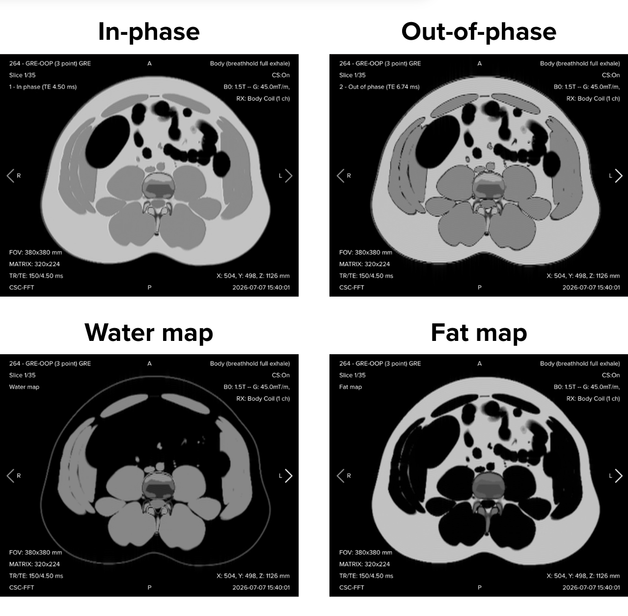
How Dixon works: The sequence acquires two echoes, one where fat and water signals are in phase and one where they are out of phase. From those, the scanner reconstructs four image sets: in-phase, out-of-phase, water-only, and fat-only.
5. Planning 3D MRCP
This is the cornerstone of the study. Everything before it establishes anatomy and context. This sequence maps the duct tree itself.
✅ Correct Planning:
Planning Instructions:
Bring the sagittal localizer back into a viewport and scroll to a slice showing the upper-abdomen organs clearly. Keep your high-resolution coronal and axial images ready for planning.
Plan the slab as a coronal. Position on the coronal T2 image, and set the in-plane position. The slab should then sit perpendicular on the axial view.
Use the axial T2 FS to check the extent of the gallbladder, then scroll down to find the common bile duct and pancreatic duct. These are the structures to cover in every case.
Use appropriate geometry parameters:
Slice number: 75–85, enough to cover the hepatobiliary system and no more. Every extra slice costs time on an already long sequence.
Slice thickness: 1.6 mm, thin near-isotropic voxels.
Slice gap: 0 mm, contiguous slices are required for a true 3D volume.
Angle the slab strategically so it captures those structures without including surrounding anatomy that adds nothing here.
Acquire with respiratory triggering. Verify the patient’s breathing is consistent, otherwise the listed scan time will stretch out significantly.
Parameters for 3D MRCP:
Parameter
Recommended Values
Why These Values
Effective Echo Time (TE)
500–800 ms
Ultra-long TE for heavy T2 weighting, so only static fluid retains signal. Higher TE means lower signal, so balance against SNR.
Repetition Time (TR)
2,500–3,000 ms
Long TR gives enough relaxation for the heavily T2-weighted readout. With respiratory triggering, the effective TR follows the breathing cycle.
Field of View (FOV)
340 × 340 mm
Focused on the hepatobiliary region rather than the whole abdomen.
Matrix
244 × 244
Combined with the FOV, gives roughly 1.4 mm in both in-plane directions, near-isotropic against the 1.6 mm slice thickness.
Foldover Direction (Phase)
Foot-to-Head (FH)
One of the two in-plane options for a coronal slab, with foldover suppression applied to limit the residual wrap.
Number of Slices
75–85
Enough to cover the biliary tree and pancreatic duct, and no more.
Slice Thickness
1.6 mm
Thin near-isotropic voxels resolve small stones and fine ducts, and allow reconstruction in any plane.
Slice Gap
0 mm
Contiguous slices are required for a true 3D volume and clean reconstructions.
NEX / Averages
1
Single average, since the sequence is already long.
Bandwidth per pixel
400–450 Hz/px
Short echo spacing matters across a 150-echo train, so bandwidth sits well above the 224 Hz/px chemical shift threshold at 1.5 T, even though that costs SNR.
Turbo Factor / ETL
140–160
Very long echo train collects the whole slice efficiently within each respiratory window.
Parallel Imaging
No
Not used here, since parallel imaging costs SNR the thin slices cannot spare.
Partial Fourier
Phase-conjugate (half-Fourier), factor 0.6
Fills 60% of k-space in the phase direction and reconstructs the rest, which is the acceleration used instead of parallel imaging.
Foldover Suppression
Yes
Limits wraparound in the FH direction.
Fat Suppression
Spectral
Suppresses background signal so only the fluid-filled ducts appear bright.
Breath-hold Mode
Free breathing
Data is collected at a consistent point in each breath, usually near end-exhalation, rather than frozen in a breath-hold.
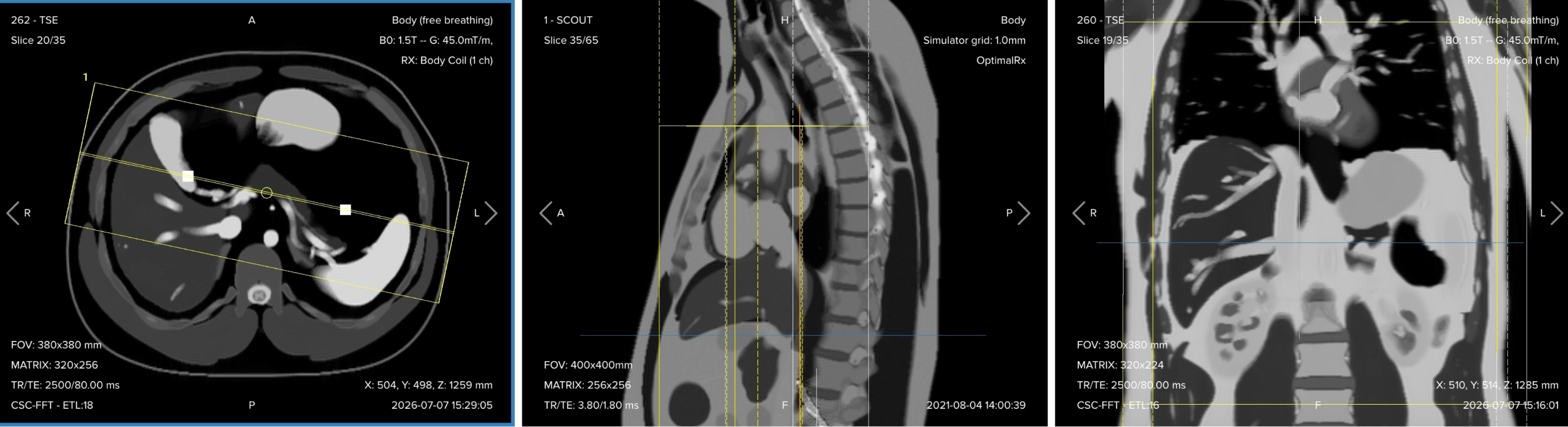
6. Planning Radial SS-TSE FS
This is a thick-slab, projection-style acquisition. Instead of a stack of parallel slices, it rotates a small number of thick slices around a single central axis.
✅ Correct Planning:
Planning Instructions:
Bring back a high-resolution coronal T2 image for planning.
Set the first slice perpendicular on the axial image and center it. That slice sits in a true coronal plane through the biliary tree.
Enable radial slices, and set the number of slices.
The slices rotate at a fixed angle around that initial position. Completing 360° gives multiple projection views of the duct tree from different angles.
Typically 9–12 slices are enough, since each views the ducts from a different angle.
Acquire as breath-holds in the same direction used on the single-shot sequence, so slice positions stay consistent.
Parameters for Radial SS-TSE FS:
Parameter
Recommended Values
Why These Values
Effective Echo Time (TE)
800–1,000 ms
Very high TE for a heavily T2-weighted projection image, similar contrast to the 3D MRCP.
Repetition Time (TR)
5,000–6,000 ms
Long TR gives full relaxation between slices for the heavily T2-weighted single-shot readout.
Field of View (FOV)
380 × 380 mm
Wide enough to keep the whole duct system inside every rotated slice.
Matrix
288 × 288
Square matrix gives roughly 1.3 mm resolution in both in-plane directions, which is needed because the slice rotates.
Foldover Direction (Phase)
Right-to-Left (RL)
Matches the coronal slice orientation.
Slice Thickness
40–45 mm
Thick slab produces a projection-style image of the whole duct system, similar to conventional cholangiography.
Number of Radial Slices
9–12
Each slice views the duct tree from a different angle through a full 360° rotation.
NEX / Averages
1
Single average, since each slice completes in roughly one to two seconds.
Bandwidth per pixel
400–450 Hz/px
Short echo spacing is what allows a single-shot readout at this echo time, so bandwidth sits well above the 224 Hz/px chemical shift threshold at 1.5 T.
Use Min. Echo Spacing
Yes
Packs the echo train as tightly as possible so each slice finishes in seconds.
Parallel Imaging
No
Not used here. The speed comes from the single-shot readout and half-Fourier instead.
Partial Fourier
Phase-conjugate (half-Fourier), factor 0.6
Fills 60% of k-space in the phase direction and reconstructs the rest, which is what makes a single shot possible at this echo time. Same approach as the 3D MRCP.
Foldover Suppression
Yes
Limits wraparound across the wide rotating field of view.
Fat Suppression
Spectral
Suppresses background fat so the bright ducts dominate the projection.
Breath-hold Mode
Exhale or inhale
Each slice completes in 1-2 seconds, but the full set of 9-12 slices takes about 45-70 seconds in total, so it is typically split across several short breath-holds. Match the direction used on the single-shot sequence.
How to Avoid Artifacts When Planning the Sequences
The table below lists the 5 common MRCP artifacts, and what techniques you can use to avoid them:
Artifact
Solution – How to Avoid It
Respiratory motion
Coach the patient on calm, regular breathing before the scan, and use respiratory or navigator-triggered 3D MRCP when available. If the 3D sequence is degraded, fall back on the fast 2D thick-slab MRCP as a motion-resistant backup.
Susceptibility (gas, clips, pneumobilia)
Cross-check any dark focus against the single-shot and 3D MRCP source images. Check for pneumobilia, clips, stents, or prior sphincterotomy before calling it a stone.
Review the finding across multiple planes and on the source images; a true stone stays within the duct on every slice. A pulsation artifact lines up with an adjacent vessel, most often the right hepatic artery at the common hepatic duct or the gastroduodenal artery at the mid CBD.
Partial volume / MIP averaging
Never rely on the thick MIP image alone. Always review the thin 3D source images, since MIP reconstruction can hide small stones or exaggerate strictures and blur.
GI fluid overlap
Fast beforehand. Use a site-approved negative oral contrast agent when local protocol allows it, such as pineapple juice, to darken bright stomach and duodenal fluid that can overlap the bile duct.
Part 3: Review the Images
Finally, we will review the images to ensure all the anatomical information we need is clear.
These key structures must be clearly visible in an MRCP:
Intrahepatic bile ducts, right and left hepatic ducts
Common hepatic duct and cystic duct
Gallbladder, including wall and contents
Common bile duct along its full length to the ampulla
Main pancreatic duct
Pancreatic parenchyma
Liver, spleen, and upper kidneys
Below, we will go through all the different image contrasts and explain their specific role in an MRCP study.
Coronal T2 TSE – Anatomical Overview of the Upper Abdomen
The coronal T2 gives a high-resolution anatomical overview of the upper abdomen, showing the liver, pancreas, gallbladder, biliary tree, and surrounding structures in a plane that runs along the axis of the biliary system.
It is valuable for detecting edema, inflammation, masses, and fluid collections, and for establishing anatomical orientation before the dedicated MRCP acquisitions.
✅ Coronal T2 TSE – Correct Image Example:
Things to Look for in Coronal T2:
Coverage runs correctly from anterior to posterior, capturing liver, gallbladder, pancreas, spleen, and upper kidneys.
The biliary tree can be traced across its general course.
No aliasing from the arms or body wall in the right-to-left direction.
Large extra-biliary masses and fluid collections are visible.
Axial T2 FS TSE – Inflammation and Edema
Suppressing the fat increases the visibility of fluid, edema, and inflammatory changes, while improving lesion detection within the liver. This sequence is particularly useful for evaluating pancreatitis, cholangitis, fluid collections, and cystic lesions, as well as gallbladder wall thickening in cholecystitis.
✅ Axial T2 FS TSE – Correct Image Example:
Things to Look for in Axial T2 FS:
Fat is uniformly suppressed across the whole field of view.
Coverage runs from the hepatic dome down to the kidneys.
Gallbladder wall thickness and any pericholecystic fluid are clearly assessable.
Peripancreatic fluid and edema stand out against the darker background.
Axial T2 SS-TSE – Fast Motion-Resistant Duct Screen
The axial T2 single-shot is a reliable overview sequence, helping identify free fluid, biliary dilatation, pancreatic abnormalities, and other upper-abdominal pathology. Because it is planned identically to the axial T2 FS, the two can be compared slice for slice.
✅ Axial T2 SS-TSE – Correct Image Example:
Things to Look for in Axial T2 SS-TSE:
Slice positions match the axial T2 FS exactly.
Images look slightly softer even though the matrix matches the axial T2 FS. That blurring comes from the long single-shot echo train and half-Fourier filling, and is the expected cost of speed.
Contrast on the vital structures remains well-defined.
Dark filling defects in the CBD are noted but confirmed on 3D MRCP source images, since flow artifact can mimic a stone.
Axial GRE Dixon – Tissue Characterization
The Dixon sequence gives tissue characterization by separating fat and water signal. It is useful for detecting hepatic steatosis, microscopic fat, adrenal adenomas, pancreatic fat infiltration, and hemorrhage, while producing high-quality fat-suppressed images. The top-left corner of the viewport shows which of the four reconstructions you are viewing.
✅ Axial GRE Dixon – Correct Image Examples (4 contrasts):
Things to Look for in Axial GRE Dixon:
In-phase: overall anatomy, acquired at the echo where fat and water signals add together.
Out-of-phase: signal drop indicating fat and water in the same voxel, pointing to steatosis or a fat-containing lesion.
Water map: completely fat-suppressed, showing only water content as bright.
Fat map: shows only the signal coming from fat.
Levels match the other axial sequences, from the top of the liver dome down to the kidneys.
3D MRCP – The Cornerstone of the Study
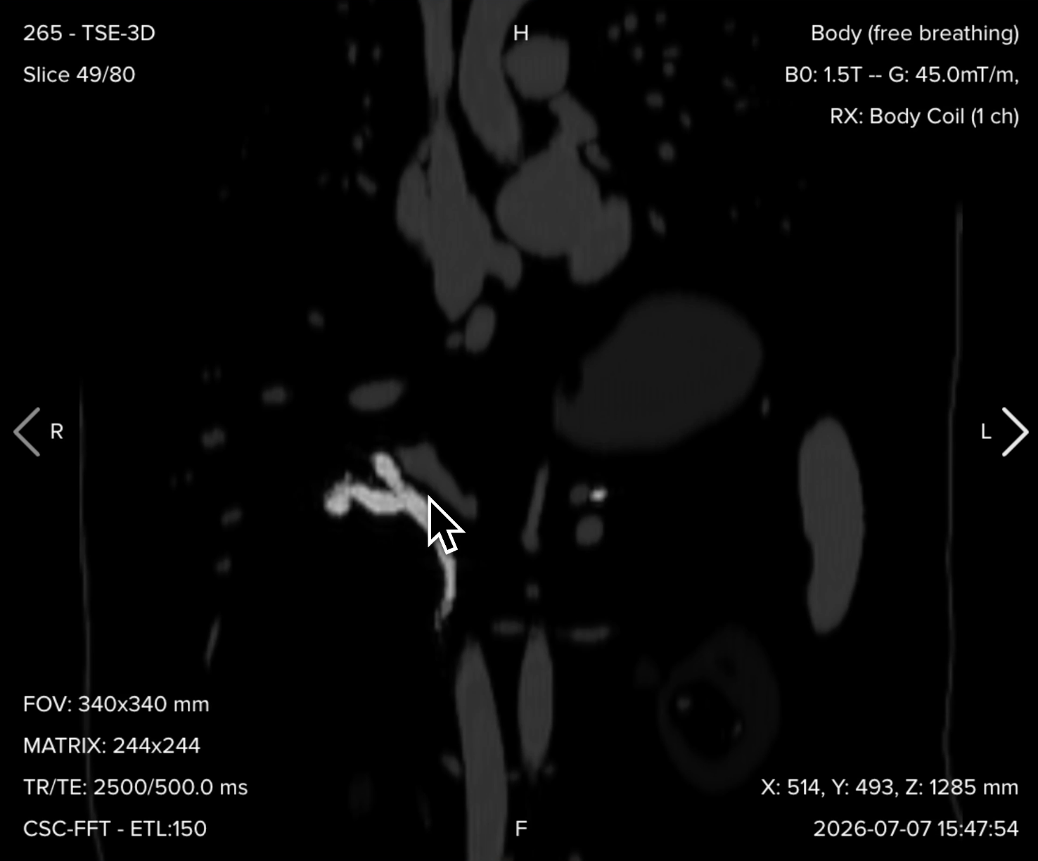
The detailed visualization of the biliary and pancreatic duct systems helps assess ductal anatomy, stones, obstructions, congenital abnormalities, ductal dilatation, and communication with cystic lesions, all without intravenous contrast.
This sequence is normally post-processed to generate MIP (maximum intensity projection) reconstructions. The native source acquisition is what you should always review first.
✅ 3D MRCP – Correct Image Example:
Things to Look for in 3D MRCP:
The full duct tree is traceable from the intrahepatic ducts to the ampulla.
The common bile duct and pancreatic duct are covered along their length.
Background signal is well suppressed, so the ducts dominate the image.
Always check the thin source images alongside the MIP. MIP reconstruction can hide small stones and exaggerate strictures.
Any apparent narrowing is cross-checked against the source images and other planes to rule out vascular pulsation from the right hepatic artery or the gastroduodenal artery.
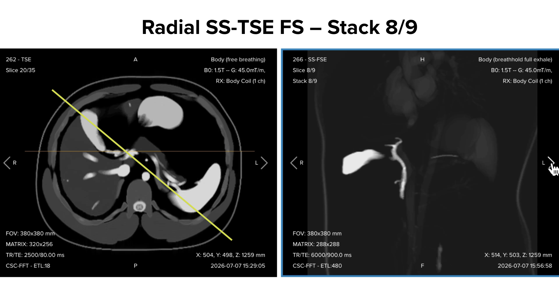
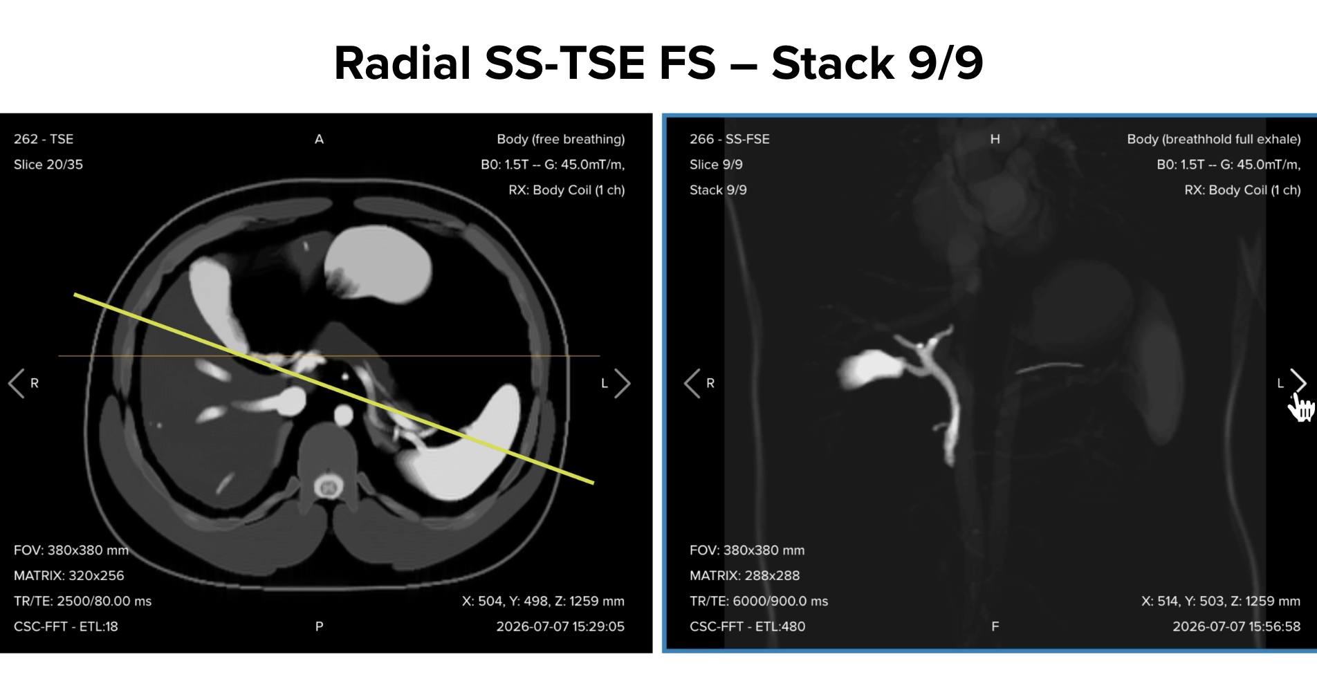
Radial SS-TSE FS – Fast Projection Backup
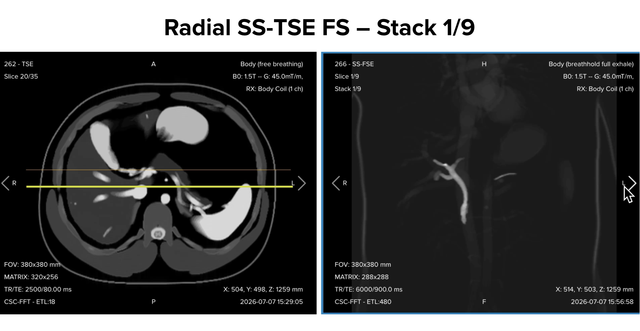
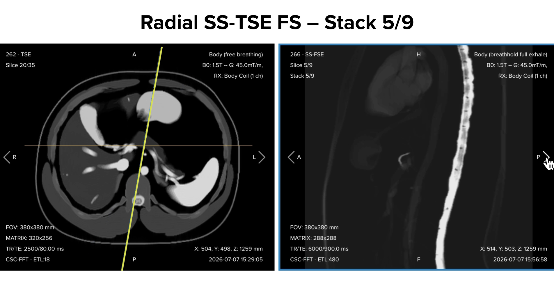
The heavily T2-weighted thick slab produces projection-like images of the biliary and pancreatic ducts. It is effective for detecting biliary obstruction, choledocholithiasis, ductal dilatation, pancreatic duct abnormalities, and gallbladder pathology, with an appearance similar to conventional cholangiography, with each slice acquired in only one to two seconds.
✅ Radial SS-TSE FS – Correct Image Examples:
Things to Look for in Radial SS-TSE FS:
The first slice is the central one, giving a true coronal view through the biliary tree.
Each following slice is rotated by a fixed angle, building a full 360° set of projection views.
The cross-reference on the axial plane shows which slice you are viewing.
Contrast is similar to the 3D MRCP, highlighting the same duct structures.
Detail is coarser than the 3D MRCP. That is the expected trade for motion resistance.
Final Checks:
Before finishing an MRCP, always check these 5 points to ensure diagnostic quality:
Complete Duct Coverage: The intrahepatic ducts, common hepatic duct, cystic duct, common bile duct to the ampulla, and main pancreatic duct must all be included on the 3D MRCP.
Motion Control: Respiratory-triggered sequences must show consistent triggering with no ghosting, and breath-hold sequences must show no blurring from a broken breath-hold.
Source Images Reviewed: Every finding on the MIP must be confirmed on the thin 3D source images, and every suspected stone on the SS-TSE must be confirmed on the 3D MRCP.
Consistent Planning: All axial sequences must sit at matching slice positions so contrasts can be compared level for level.
Image Quality and Artifacts: Fat suppression must be uniform, background GI fluid adequately dark, and there must be no significant chemical shift, wraparound, or susceptibility artifacts.

.svg)