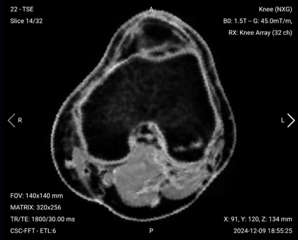
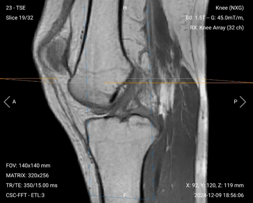
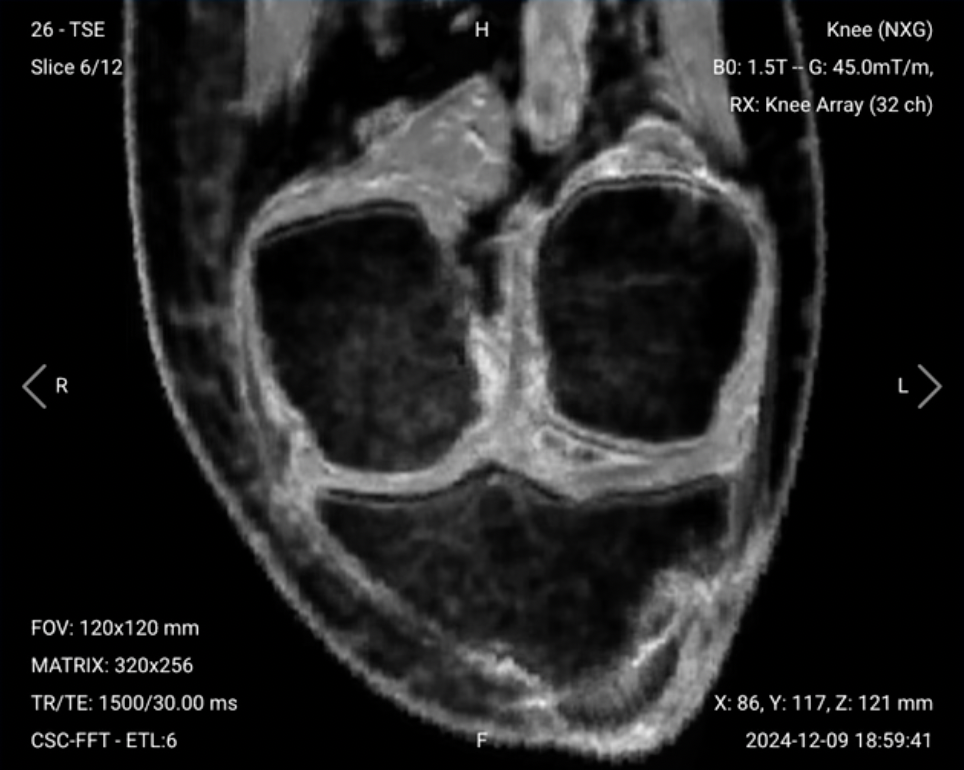
This step-by-step guide is for MRI students, radiographers and technologists who wish to improve their planning skills and master the knee MRI protocol.
What you will learn:
Key factors in knee MRIs, including trade-offs.
Patient and scanner setup tips.
Best pulse sequences and planning techniques.
Ways to avoid common artifacts.
What great knee images should look like.
Key Takeaways
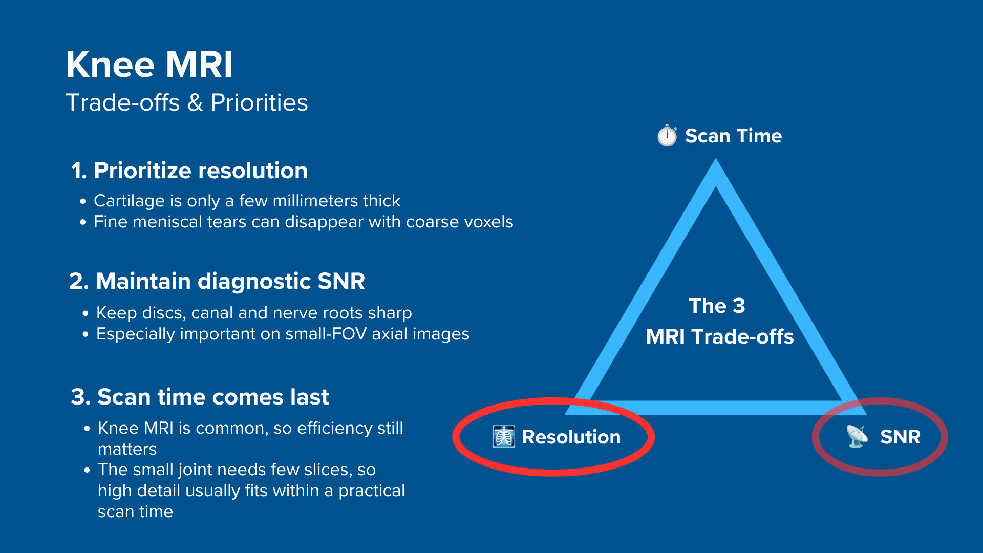
Because the knee is a small region with thin structures, it's recommended to prioritize resolution.
The findings that decide a knee report are only millimeters across, and a knee scan can usually be completed relatively quickly, so we rarely need to shorten it further. We should therefore 1) prioritize resolution, 2) maintain strong SNR for clarity, and 3) optimize scan time as needed.
We mainly use Proton Density Fat-Saturated (PD FS) sequences in knee MRIs.
PD FS sequences provide excellent soft tissue contrast, helping us see the joint structures, ligaments, and cartilage clearly. They also highlight fluids while suppressing fat signal, letting us detect fluid-related abnormalities like edema or inflammation.
Avoid these 6 common knee artifacts.
Artifacts
Solution – How to Avoid It
Chemical shift artifacts
Increase the bandwidth per pixel to reduce the spatial displacement between fat and water signals.
Wrap-around artifacts
Activate foldover suppression to prevent anatomy outside the field of view from overlapping.
Flow artifacts
Set the phase-encoding direction to steer the artifact away from the joint: superior-inferior on sagittal and coronal, right-left on axial. The cropped ACL sagittal uses anterior-posterior, due to its smaller field of view.
Motion artifacts
Shorten the scan time to reduce the risk of patient motion.
Truncation artifacts
Increase the resolution to capture more frequency information and reduce Gibbs ringing at tissue boundaries.
Susceptibility artifacts
Use Metal Artifact Reduction Sequences (MARS). Susceptibility artifacts in the knee are mostly caused by metal implants.
Intro to Knee MRIs
The knee is a complex joint we use daily for many activities: walking, running, and moving with stability. It absorbs impact, supports body weight, and enables a wide range of motion.
Because of its high use and susceptibility to injuries, the knee is one of the most frequently examined areas in MRI. Imaging helps assess ligament tears, cartilage damage, and other conditions affecting mobility and function.
In MRI, we always face a trade-off between 3 key metrics:
Scan Time: How fast a pulse sequence can be completed.
Resolution: How much detail the image can display.
SNR: How clear the image is, meaning how much signal we have compared with noise.
Improving one of these metrics often reduces the performance of the others. To decide what trade-offs to make, we must consider the needs of each clinical situation.
For knee MRIs, we face these challenges:
Cartilage is only a few millimeters thick, and a meniscal tear can be a hairline of signal barely wider than a voxel. Low resolution averages it away entirely.
High resolution means small voxels, and small voxels cost signal. We need enough SNR to separate cartilage, fluid, and ligament.
Knee MRI is frequently requested, which usually argues for a short slot. But the joint is small and needs few slices, so a full protocol still fits without cutting detail.
Therefore, we typically:
Prioritize resolution, since a tear thinner than the voxel averages away no matter how good the rest of the image is.
Maintain enough SNR to keep that resolution diagnostic, buying it back with an extra average where needed.
Optimize scan time last, since a knee scan can usually be completed quickly enough that we do not have to buy time by giving up detail.
Note! Prioritizing resolution in knee MRIs is only a general guideline, NOT a strict rule. If the patient cannot hold still, scan time moves higher in the priority order, because a blurred high-resolution acquisition is less useful than a sharp acquisition at slightly lower resolution. The right balance always depends on factors such as field strength, patient cooperation, available hardware, and the clinical question.
Knee Health Conditions and the MRI Sequences That Reveal Them
The knee MRI study can help us diagnose a wide range of health conditions. The table below lists some of the most common conditions, and what pulse sequences that reveal them:
Provides high soft-tissue contrast while suppressing fat, making it the primary sequence for ligament, meniscal and cartilage assessment.
Fat suppression makes edema and trauma stand out without fat signal interference.
Bone Lesions and Tumors:
• Bone tumors
• Bone cysts
• Osteochondritis dissecans
T1
Highlights bone marrow structure and fat, making it ideal for detecting tumors, cysts, and chronic bone lesions.
Provides high contrast between normal and abnormal bone.
Optimized for assessing the anterior cruciate ligament (ACL) with high-resolution imaging to detect subtle ligament injuries.
Fat suppression enhances contrast, improving detection of partial tears.
How to Perform a Knee MRI
The step-by-step guide below will show you how to set up and perform a knee MRI protocol in practice.
We will perform the protocol in 3 parts:
Set up the Patient and MRI Scanner
Plan and Acquire the Protocol Sequences
Review the Images
Part 1: Set up the Patient and MRI Scanner
1. Position the Patient in the Scanner
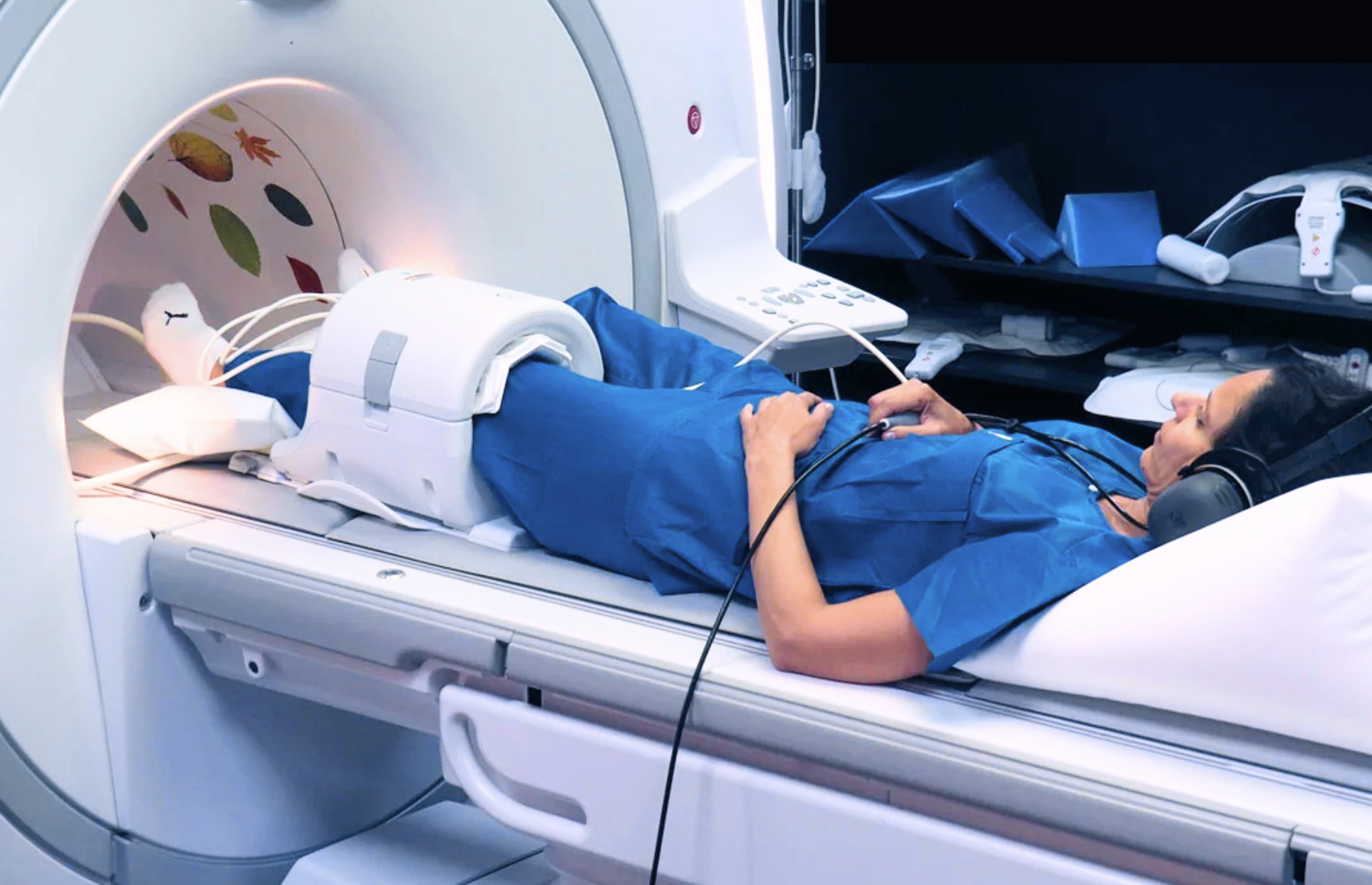
Lay the patient feet-first and supine (on their back) with the knee centered at the scanner's isocenter.
Positioning the patient feet-first can improve comfort and reduce the risk of motion, especially for those who feel anxious in enclosed spaces.
Use a dedicated knee coil array, positioned around the knee being examined. It gives full coverage of the joint, including cartilage, ligaments, and menisci, and the signal reception high-resolution imaging needs.
Once the patient is in place, review your scanner's hardware settings.
In this guide, we will use the following settings:
Scanner Setting
Value
Why This Value
Magnetic field strength
1.5 T
The most common clinical field strength, giving enough SNR for this protocol with less susceptibility and B1 artifact than 3 T. The lower susceptibility also helps around knee hardware.
Maximum gradient strength
45 mT/m
Provides strong, versatile gradient performance that supports fast imaging and precise spatial encoding.
This hardware setup is widely used in clinical practice. It balances acquisition time, image quality, and patient comfort.
3. Capture the Initial Localizer Images
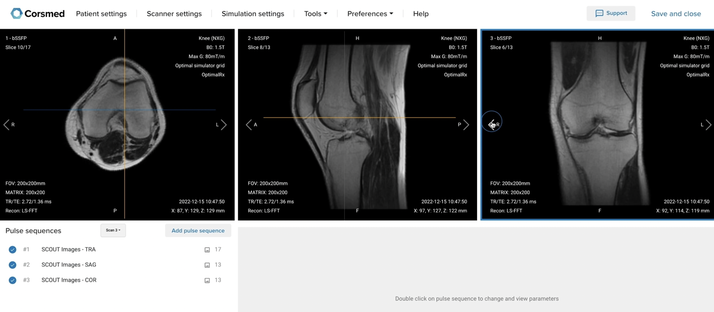
Before we can perform any MRI protocol, we must always capture initial localizer images of the patient. These images act as a guide for planning the detailed scans we will perform next.
We should always capture localizers in three planes:
Axial
Sagittal
Coronal
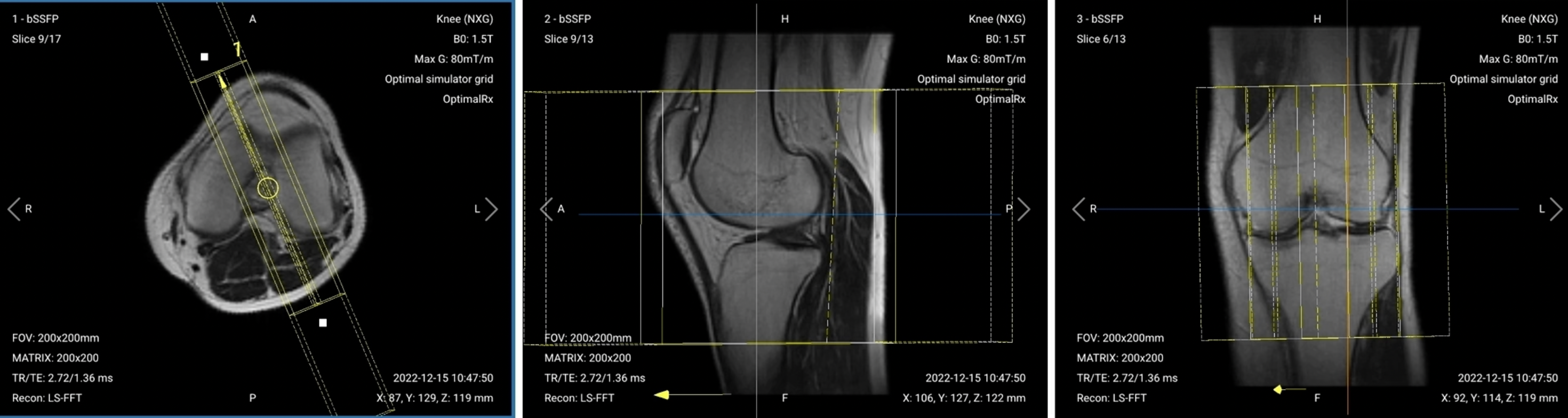
Once acquired, load the initial localizer images into the three viewports.
Then, scroll through each of the image stacks to locate a central slice that clearly shows the anatomy of the knee.
✅ Correct Setup of Localizer Images for Knee MRI:
Part 2: Plan and Acquire the Protocol Sequences
When all preparations are ready, we can start planning and acquiring the protocol sequences.
Let's go through the pulse sequences that a standard knee MRI protocol includes, why we perform them, and how to set them up.
The 7 Sequences of a Standard Knee MRI
Sagittal PD FS
Coronal PD FS
Axial PD FS
Sagittal T1 TSE
Coronal T2 TSE
Sagittal PD FS ACL (Anterior Cruciate Ligament)
Coronal PD FS ACL
We mainly use PD FS sequences for this study. This type of sequence provides excellent soft tissue contrast, which helps us see the knee's joint structures, ligaments, and cartilage clearly. PD FS also highlights fluids while suppressing signal from fat, letting us detect fluid-related abnormalities like edema or inflammation.
Note: Your facility may have its own local policies, so the protocol might differ in some of these sequences. If they differ, then always follow your own institution's guidelines.
The values in the tables below are worked examples for the 1.5 T setup used in this guide. Exact numbers vary by scanner, coil and department, so treat them as a starting point rather than as fixed limits.
In the sections below, we go through how to plan and set up each sequence.
1. Sagittal PD FS
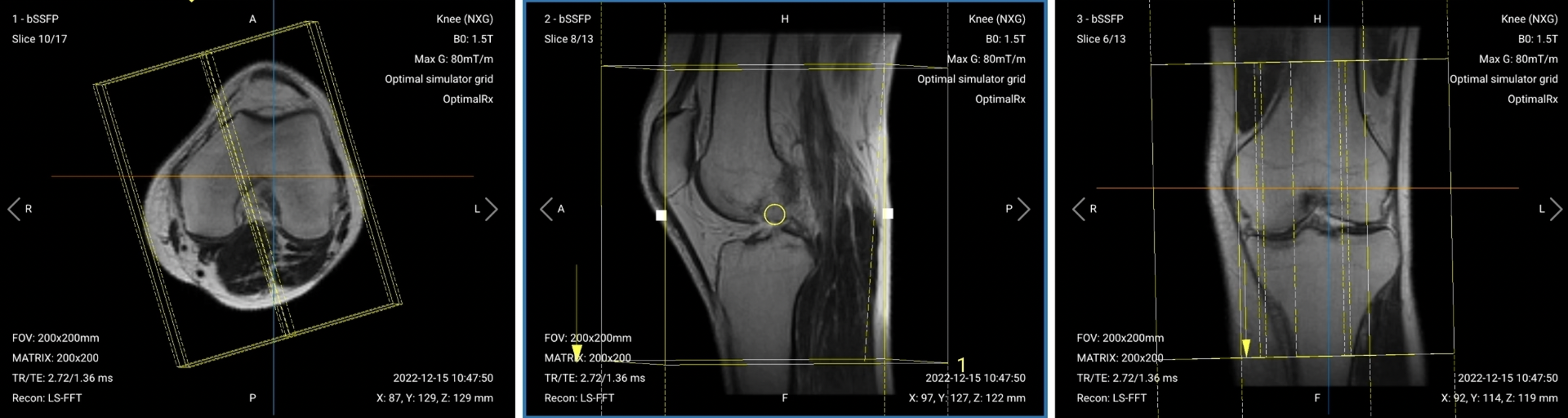
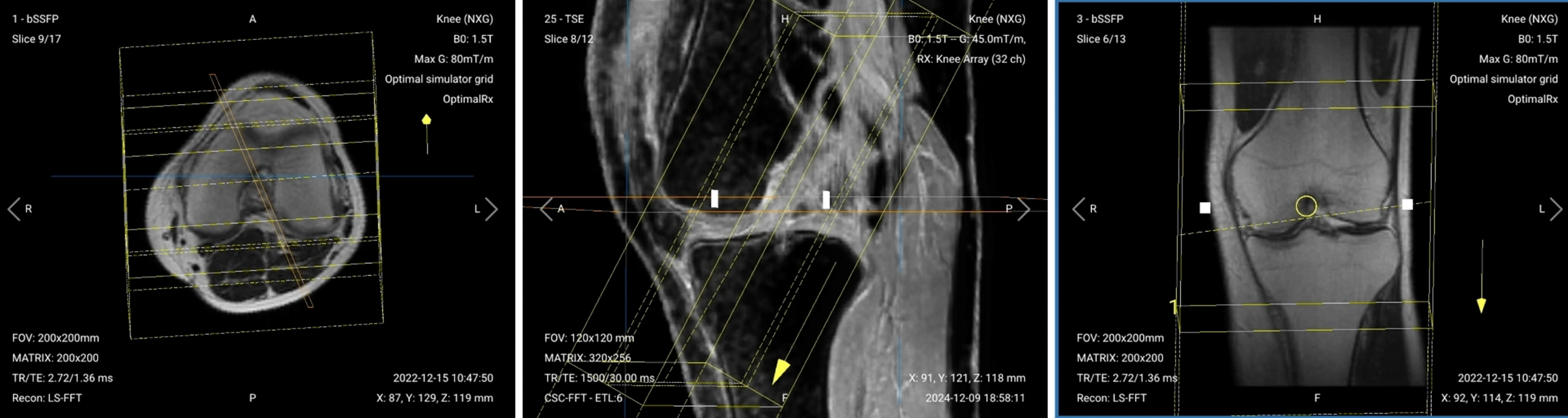
✅ Correct Planning:
Planning Instructions:
Use the lateral condyle of the femur as the anatomical reference.
Set the slice angulation as follows:
Axial Localizer: Parallel to the lateral condyle of the femur.
Coronal Localizer: Parallel to the midline of the femur and tibia.
Check on the sagittal localizer that the resulting plane runs parallel to the anterior cruciate ligament, which lies parallel to the lateral condyle.
Add enough slices to fully cover the knee from medial to lateral.
Center the slices and adjust the slice thickness and gap for optimal spatial resolution.
Parameters for Sagittal PD FS:
Parameter
Recommended Values
Why These Values
Echo Time (TE)
20–40 ms
Short TE is required for PD contrast.
Repetition Time (TR)
1,600–2,000 ms
Long TR is required for PD contrast.
Field of View (FOV)
140 x 140 mm
Small enough to focus on the knee region.
Matrix
320 x 256
Gives ~0.44 x 0.55 mm resolution, enough to resolve cartilage, menisci, and ligaments.
Foldover Direction (Phase)
Foot-to-Head (FH), along the superior-inferior axis
Places pulsation ghosts from the popliteal artery along the vessel's own course, rather than across the joint.
Number of Slices
30–34
Enough slices to cover the knee from medial to lateral.
Slice Thickness
3 mm
Thin enough to limit partial volume averaging across the menisci and cartilage, at some cost in signal per slice.
Slice Gap
0.3 mm
10% of slice thickness, which limits cross-talk without hiding anatomy.
NEX / Averages
1
To get enough SNR, while keeping scan time short.
Turbo Factor / ETL
4–8
Limits T2 decay across the echo train, preserving fine-detail sharpness.
Parallel Imaging
No
The sequence already fits its scan time, so there is nothing to gain by trading SNR for acceleration.
Partial Fourier
No
Full k-space is acquired, since the SNR matters more here than the time a partial acquisition would save.
Bandwidth per pixel
250–350 Hz/px
High enough to limit chemical shift, while keeping the SNR this sequence needs.
Foldover Suppression
Yes
To avoid aliasing or wrap-around artifacts.
Fat Suppression
Spectral
To make soft tissues, cartilage, and fluid-related abnormalities in the knee more visible.
2. Coronal PD FS
✅ Correct Planning:
Planning Instructions:
Use the medial and lateral condyles of the femur as the anatomical reference.
Align the slices as follows:
Axial Localizer: Parallel to the medial and lateral condyles of the femur.
Sagittal Localizer: Parallel to the midline of the femur and tibia.
Add enough slices to cover the knee from anterior to posterior.
Center the slices and adjust the slice thickness and gap for optimal spatial resolution.
Parameters for Coronal PD FS:
Parameter
Recommended Values
Why These Values
Echo Time (TE)
20–40 ms
Short TE is required for PD contrast.
Repetition Time (TR)
1,600–2,000 ms
Long TR is required for PD contrast.
Field of View (FOV)
140 x 140 mm
Small enough to focus on the knee region.
Matrix
320 x 256
Gives ~0.44 x 0.55 mm resolution, enough to resolve cartilage, menisci, and ligaments.
Foldover Direction (Phase)
Foot-to-Head (FH), along the superior-inferior axis
Keeps popliteal pulsation ghosting in the superior-inferior direction, away from the collateral ligaments and menisci.
Number of Slices
30–34
Enough slices to cover the knee from anterior to posterior.
Slice Thickness
3 mm
Thin enough to limit partial volume averaging across the menisci and cartilage, at some cost in signal per slice.
Slice Gap
0.3 mm
10% of slice thickness, which limits cross-talk without hiding anatomy.
NEX / Averages
1
To get enough SNR, while keeping scan time short.
Turbo Factor / ETL
4–8
Limits T2 decay across the echo train, preserving fine-detail sharpness.
Parallel Imaging
No
The sequence already fits its scan time, so there is nothing to gain by trading SNR for acceleration.
Partial Fourier
No
Full k-space is acquired, since the SNR matters more here than the time a partial acquisition would save.
Bandwidth per pixel
250–350 Hz/px
High enough to limit chemical shift, while keeping the SNR this sequence needs.
Foldover Suppression
Yes
To avoid aliasing or wrap-around artifacts.
Fat Suppression
Spectral
To make soft tissues, cartilage, and fluid-related abnormalities in the knee more visible.
3. Axial PD FS
✅ Correct Planning:
Planning Instructions:
Use the femur, tibia, and meniscus as anatomical references.
Align the slices as follows:
Sagittal Localizer: Perpendicular to the femur and tibia, and parallel to the menisci.
Coronal Localizer: Parallel to the lateral and medial condyles of the femur.
Add enough slices to cover the knee joint, from the patella's border (upper part of the knee) down to the tibial tuberosity.
Center the slices and adjust the slice thickness and gap for optimal spatial resolution.
Parameters for Axial PD FS:
Parameter
Recommended Values
Why These Values
Echo Time (TE)
20–40 ms
Short TE is required for PD contrast.
Repetition Time (TR)
1,600–2,000 ms
Long TR is required for PD contrast.
Field of View (FOV)
140 x 140 mm
Small enough to focus on the knee region.
Matrix
320 x 256
Gives ~0.44 x 0.55 mm resolution, enough to resolve cartilage, menisci, and ligaments.
Foldover Direction (Phase)
Right-to-Left (RL), along the left-right axis
On axial slices, right-left steers popliteal pulsation off the patellofemoral joint.
Number of Slices
30–34
Enough slices to cover the joint from the border of the patella down to the tibial tuberosity.
Slice Thickness
3 mm
Thin enough to limit partial volume averaging across the menisci and cartilage, at some cost in signal per slice.
Slice Gap
0.3 mm
10% of slice thickness, which limits cross-talk without hiding anatomy.
NEX / Averages
1
To get enough SNR, while keeping scan time short.
Turbo Factor / ETL
4–8
Limits T2 decay across the echo train, preserving fine-detail sharpness.
Parallel Imaging
No
The sequence already fits its scan time, so there is nothing to gain by trading SNR for acceleration.
Partial Fourier
No
Full k-space is acquired, since the SNR matters more here than the time a partial acquisition would save.
Bandwidth per pixel
250–350 Hz/px
High enough to limit chemical shift, while keeping the SNR this sequence needs.
Foldover Suppression
Yes
To avoid aliasing or wrap-around artifacts.
Fat Suppression
Spectral
To make soft tissues, cartilage, and fluid-related abnormalities in the knee more visible.
4. Sagittal T1 TSE
✅ Correct Planning:
Planning Instructions:
Copy the slice geometry and planning from the sagittal PD FS sequence.
Keep the same slice angulation, coverage, and positioning so images of different contrasts can be compared directly.
Parameters for Sagittal T1 TSE:
Parameter
Recommended Values
Why These Values
Echo Time (TE)
10–20 ms
Short TE is required for T1 contrast.
Repetition Time (TR)
300–500 ms
Short TR is required for T1 contrast.
Field of View (FOV)
140 x 140 mm
Small enough to focus on the knee region.
Matrix
320 x 256
Gives ~0.44 x 0.55 mm resolution, enough to resolve cartilage, menisci, and ligaments.
Foldover Direction (Phase)
Foot-to-Head (FH), along the superior-inferior axis
Places pulsation ghosts from the popliteal artery along the vessel's own course, rather than across the joint.
Number of Slices
30–34
Matches the sagittal PD FS coverage from medial to lateral.
Slice Thickness
3 mm
Thin enough to limit partial volume averaging across the menisci and cartilage, at some cost in signal per slice.
Slice Gap
0.3 mm
10% of slice thickness, which limits cross-talk without hiding anatomy.
NEX / Averages
1
To get enough SNR, while keeping scan time short.
Turbo Factor / ETL
2–4
Kept short so the effective TE stays short, preserving T1-weighting.
Parallel Imaging
No
The sequence already fits its scan time, so there is nothing to gain by trading SNR for acceleration.
Partial Fourier
No
Full k-space is acquired, since the SNR matters more here than the time a partial acquisition would save.
Bandwidth per pixel
250–350 Hz/px
High enough to limit chemical shift, while keeping the SNR this sequence needs.
Foldover Suppression
Yes
To avoid aliasing or wrap-around artifacts.
Fat Suppression
None
Not needed; bright fat is what makes this sequence useful.
5. Coronal T2 TSE
✅ Correct Planning:
Planning Instructions:
Copy the slice geometry and planning from the coronal PD FS sequence.
Keep the same slice angulation, coverage, and positioning so images of different contrasts can be compared directly.
Parameters for Coronal T2 TSE:
Parameter
Recommended Values
Why These Values
Echo Time (TE)
80–120 ms
Long TE is required for T2 contrast.
Repetition Time (TR)
2,500–4,000 ms
Long TR is required for T2 contrast.
Field of View (FOV)
140 x 140 mm
Small enough to focus on the knee region.
Matrix
320 x 256
Gives ~0.44 x 0.55 mm resolution, enough to resolve cartilage, menisci, and ligaments.
Foldover Direction (Phase)
Foot-to-Head (FH), along the superior-inferior axis
Keeps popliteal pulsation ghosting in the superior-inferior direction, away from the collateral ligaments and menisci.
Number of Slices
30–34
Matches the coronal PD FS coverage from anterior to posterior.
Slice Thickness
3 mm
Thin enough to limit partial volume averaging across the menisci and cartilage, at some cost in signal per slice.
Slice Gap
0.3 mm
10% of slice thickness, which limits cross-talk without hiding anatomy.
NEX / Averages
1
To get enough SNR, while keeping scan time short.
Turbo Factor / ETL
15–20
Higher turbo factor reduces scan time, and long effective TE provides T2 weighting.
Parallel Imaging
No
The sequence already fits its scan time, so there is nothing to gain by trading SNR for acceleration.
Partial Fourier
No
Full k-space is acquired, since the SNR matters more here than the time a partial acquisition would save.
Bandwidth per pixel
250–350 Hz/px
High enough to limit chemical shift, while keeping the SNR this sequence needs.
Foldover Suppression
Yes
To avoid aliasing or wrap-around artifacts.
Fat Suppression
None
Not used here; marrow edema is assessed on the PD FS sequences instead.
Use the axial localizer to identify the anterior cruciate ligament (ACL).
Set the slice angulation parallel to the ACL on the axial localizer.
Check on the sagittal localizer that the plane follows the ligament along its length.
Set a thinner slice thickness and gap for high-resolution ligament imaging.
Limit the number of slices to cover only the ligament. Then, center the slice package.
Parameters for Sagittal PD FS ACL:
Parameter
Recommended Values
Why These Values
Echo Time (TE)
20–40 ms
Short TE is required for PD contrast.
Repetition Time (TR)
1,300–1,700 ms
Long TR is required for PD contrast.
Field of View (FOV)
120 x 120 mm
Tighter FOV cropped to the ligament, for higher resolution.
Matrix
320 x 256
Gives ~0.38 x 0.47 mm resolution, enough to separate partial tears from intact ligament.
Foldover Direction (Phase)
Anterior-to-Posterior (AP)
At this tight field of view the leg extends beyond the field superior-inferior, so the phase axis runs anterior-posterior instead.
Number of Slices
10–14
Only enough slices to span the ligament and its immediate margins.
Slice Thickness
2 mm
Thin enough to follow the ACL fibers without partial volume from the intercondylar roof, at some cost in signal per slice.
Slice Gap
0.2 mm
10% of slice thickness, which limits cross-talk without hiding anatomy.
NEX / Averages
1
To get enough SNR, while keeping scan time short.
Turbo Factor / ETL
4–8
Limits T2 decay across the echo train, preserving fine-detail sharpness.
Parallel Imaging
No
The sequence already fits its scan time, so there is nothing to gain by trading SNR for acceleration.
Partial Fourier
No
Full k-space is acquired, since the SNR matters more here than the time a partial acquisition would save.
Bandwidth per pixel
250–350 Hz/px
High enough to limit chemical shift, while keeping the SNR this sequence needs.
Foldover Suppression
Yes
To avoid aliasing or wrap-around artifacts.
Fat Suppression
Spectral
To make soft tissues, cartilage, and fluid-related abnormalities in the knee more visible.
7. Coronal PD FS ACL
✅ Correct Planning:
Planning Instructions:
Use the previous sagittal PD FS ACL image for planning.
Align the slices as follows:
Sagittal Localizer: Parallel to the ACL, from its origin to insertion.
Coronal Localizer: Parallel to the ACL, using the reconstructed sagittal PD FS ACL image to confirm the angle.
Set thin slice thickness and gap for high-resolution imaging.
Limit the number of slices to cover only the ligament. Then, center the slice package.
Parameters for Coronal PD FS ACL:
Parameter
Recommended Values
Why These Values
Echo Time (TE)
20–40 ms
Short TE is required for PD contrast.
Repetition Time (TR)
1,300–1,700 ms
Long TR is required for PD contrast.
Field of View (FOV)
120 x 120 mm
Tighter FOV cropped to the ligament, for higher resolution.
Matrix
320 x 256
Gives ~0.38 x 0.47 mm resolution, enough to separate partial tears from intact ligament.
Foldover Direction (Phase)
Foot-to-Head (FH), along the superior-inferior axis
Keeps popliteal pulsation ghosting in the superior-inferior direction, away from the ligament.
Number of Slices
10–14
Only enough slices to span the ligament and its immediate margins.
Slice Thickness
2 mm
Thin enough to follow the ACL fibers without partial volume from the intercondylar roof, at some cost in signal per slice.
Slice Gap
0.2 mm
10% of slice thickness, which limits cross-talk without hiding anatomy.
NEX / Averages
1
To get enough SNR, while keeping scan time short.
Turbo Factor / ETL
4–8
Limits T2 decay across the echo train, preserving fine-detail sharpness.
Bandwidth per pixel
250–350 Hz/px
High enough to limit chemical shift, while keeping the SNR this sequence needs.
Parallel Imaging
No
The sequence already fits its scan time, so there is nothing to gain by trading SNR for acceleration.
Partial Fourier
No
Full k-space is acquired, since the SNR matters more here than the time a partial acquisition would save.
Foldover Suppression
Yes
To avoid aliasing or wrap-around artifacts.
Fat Suppression
Spectral
To make soft tissues, cartilage, and fluid-related abnormalities in the knee more visible.
How to Avoid Artifacts When Planning the Sequences
The table below lists the 6 common knee artifacts, and what techniques you can use to avoid them:
Artifacts
Solution – How to Avoid It
Chemical shift artifacts
Increase the bandwidth per pixel to reduce the spatial displacement between fat and water signals.
Wrap-around artifacts
Activate foldover suppression to prevent anatomy outside the field of view from overlapping.
Flow artifacts
Set the phase-encoding direction to steer the artifact away from the joint: superior-inferior on sagittal and coronal, right-left on axial. The cropped ACL sagittal uses anterior-posterior, due to its smaller field of view.
Motion artifacts
Shorten the scan time to reduce the risk of patient motion.
Truncation artifacts
Increase the resolution to capture more frequency information and reduce Gibbs ringing at tissue boundaries.
Susceptibility artifacts
Use Metal Artifact Reduction Sequences (MARS). Susceptibility artifacts in the knee are mostly caused by metal implants.
Part 3: Review the Images
Finally, we will review the images to ensure all the anatomical information we need is clear.
These key structures must be clearly visible in a knee MRI:
Articular cartilage of the femur, tibia, and patella
Menisci (medial and lateral)
Ligaments, including ACL, PCL, MCL, and LCL
Tendons, including quadriceps and patellar tendons
Synovial fluid and joint capsule
Bone marrow and surrounding soft tissues
Below, we will go through all the different image contrasts and explain their specific role in imaging the knee.
PD FS – Best for Soft Tissues, Cartilage, and Fluid-Sensitive Pathologies
PD FS imaging provides high contrast between soft tissues while suppressing fat, making it ideal for evaluating joint structures.
In knee MRI, PD FS is the primary sequence for detecting ligament injuries, meniscal tears, and cartilage damage. It allows for a detailed evaluation of bone marrow edema, tendonitis, and synovial inflammation, making it the core sequence for both traumatic and degenerative conditions.
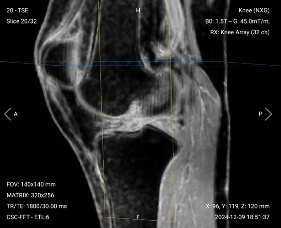
✅ Sagittal PD FS of the Knee – Correct Image:
The sagittal PD FS sequence provides a side view of the knee, which lets us:
Assess the ACL and PCL in detail for fiber integrity and partial or full tears.
Visualize menisci from anterior to posterior horns.
Evaluate the patellar and quadriceps tendons.
Detect bone marrow edema in the femoral condyles and tibial plateau.
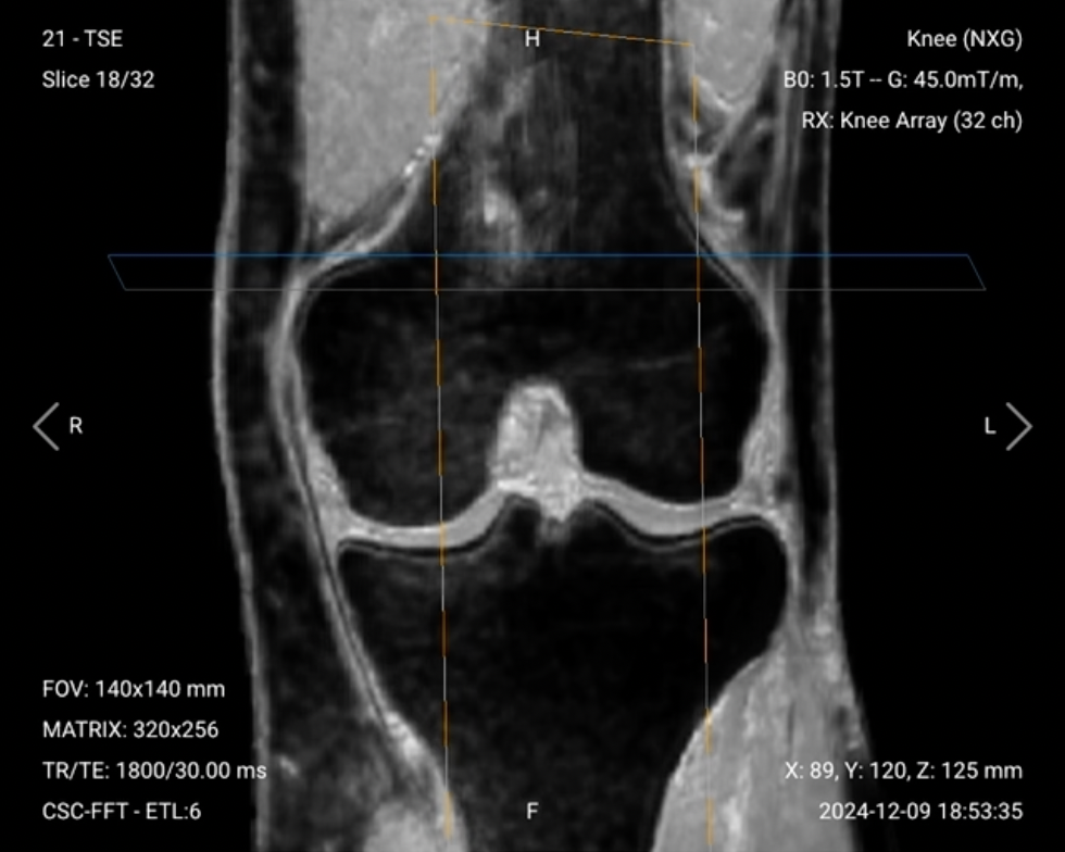
✅ Coronal PD FS of the Knee – Correct Image:
Viewed from the front, the coronal PD FS shows:
Medial and lateral menisci, ideal for detecting horizontal or radial tears.
Collateral ligaments (MCL & LCL) for sprains, tears, or thickening.
Bone marrow signal changes, including stress fractures or contusions.
✅ Axial PD FS of the Knee – Correct Image:
The axial PD FS sequence provides a top-down view, useful for:
Patellofemoral cartilage damage and signs of patellar malalignment such as tilt or lateral subluxation in the trochlear groove.
Joint effusion and synovial thickening.
Patellar retinacula and the popliteal fossa, including cyst formation and soft tissue swelling.
T1 TSE – Highlight Fat-Containing Tissues and Structural Abnormalities
T1-weighted imaging makes fat appear bright and fluid dark. This contrast is ideal for fat-rich tissues and structural abnormalities. T1 shows anatomical structures clearly, since it helps us see where different solid tissues like muscle and fat meet.
In knee MRI, T1 sequences are used to evaluate bone marrow, fractures, and fatty structures such as Hoffa's fat pad. T1 is also useful for detecting subacute hemorrhage, osteonecrosis, and tumors because it differentiates normal fatty marrow from pathological changes.
✅ Sagittal T1 of the Knee – Correct Image:
On the sagittal T1, look for:
Bone marrow composition, where loss of normal fatty marrow signal points to fractures or marrow replacement. Suspected edema is mapped on the fat-saturated PD sequences.
Meniscal morphology and outline, which complements the PD FS sequences where internal signal change is actually assessed.
Structural integrity of ligaments when compared with PD FS sequences.
T2 TSE – Highlight Fluid-Related Tissues and Conditions
T2-weighted imaging makes fluids appear bright. This contrast is ideal to detect tissues and abnormalities associated with high water content.
In knee MRI, T2 sequences are well suited to assessing joint effusion, meniscal cysts, synovitis, and cartilage defects. Because this sequence is acquired without fat suppression, bright marrow fat can mask edema, so marrow signal changes are read from the fat-saturated PD sequences.
✅ Coronal T2 of the Knee – Correct Image:
The coronal T2 is where to read:
Joint effusion and synovitis in the medial and lateral compartments.
Cystic changes in menisci, including meniscal cyst formation.
Cartilage defects in weight-bearing areas of the femur and tibia.
PD FS ACL – Focused ACL Imaging for Ligament Integrity
A dedicated PD FS sequence for the ACL is optimized to evaluate ligament fiber continuity, partial tears, and ligament edema. It allows for a more detailed view of ligamentous injuries, bone bruising, and secondary stabilizers.
In knee MRI, PD FS ACL sequences help identify partial or full-thickness ACL tears, fiber disruptions, and associated bone marrow edema from trauma. These focused series improve visualization of ACL fiber continuity and support pre-surgical planning, alongside the standard multiplanar sequences.
✅ Sagittal PD FS ACL – Correct Image:
The sagittal PD FS ACL sequence provides a direct look at the ACL, showing:
ACL fiber integrity, including partial vs. complete tears.
Bone marrow bruising patterns in the lateral femoral condyle and tibial plateau.
Deep lateral femoral notch sign, a deepened condylopatellar sulcus that suggests an impaction injury from ACL rupture.
✅ Coronal PD FS ACL – Correct Image:
The coronal PD FS ACL sequence provides an alternative angle of the ACL, helping assess:
ACL orientation, in relation to the lateral femoral condyle.
Segond fracture, an avulsion at the lateral tibial rim that is strongly associated with ACL rupture.
Meniscotibial ligament injuries, often associated with ACL tears.
Final Checks
Before finishing a knee MRI, always check these 5 points to ensure diagnostic quality:
Ligaments and Menisci: ACL, PCL, MCL, LCL, and both menisci must be clearly visible and sharply defined in PD FS sequences.
Cartilage and Joint Surfaces: Articular cartilage of the femur, tibia, and patella must appear smooth and intact; look for thinning or defects.
Field of View and Coverage: The five main-region sequences must cover from the border of the patella down to the tibial tuberosity, including the posterior structures. The two dedicated ACL sequences are deliberately restricted to the ligament and are checked for full origin-to-insertion coverage instead.
Fat Suppression Quality: PD FS sequences must show uniform fat suppression so edema and fluid appear clearly.
Image Quality and Artifacts: Images must have strong SNR, crisp detail, and no wrap-around, chemical shift, or motion artifacts.

.svg)