This step-by-step guide is for MRI students, radiographers, and technologists who wish to improve their planning skills and master the internal auditory canal (IAC/IAM) MRI protocol.
What you will learn:
Key factors in IAC/IAM MRIs, including trade-offs.
Patient and scanner setup tips.
Best pulse sequences and planning techniques.
Ways to avoid common artifacts.
What great IAC/IAM images should look like.
Key Takeaways
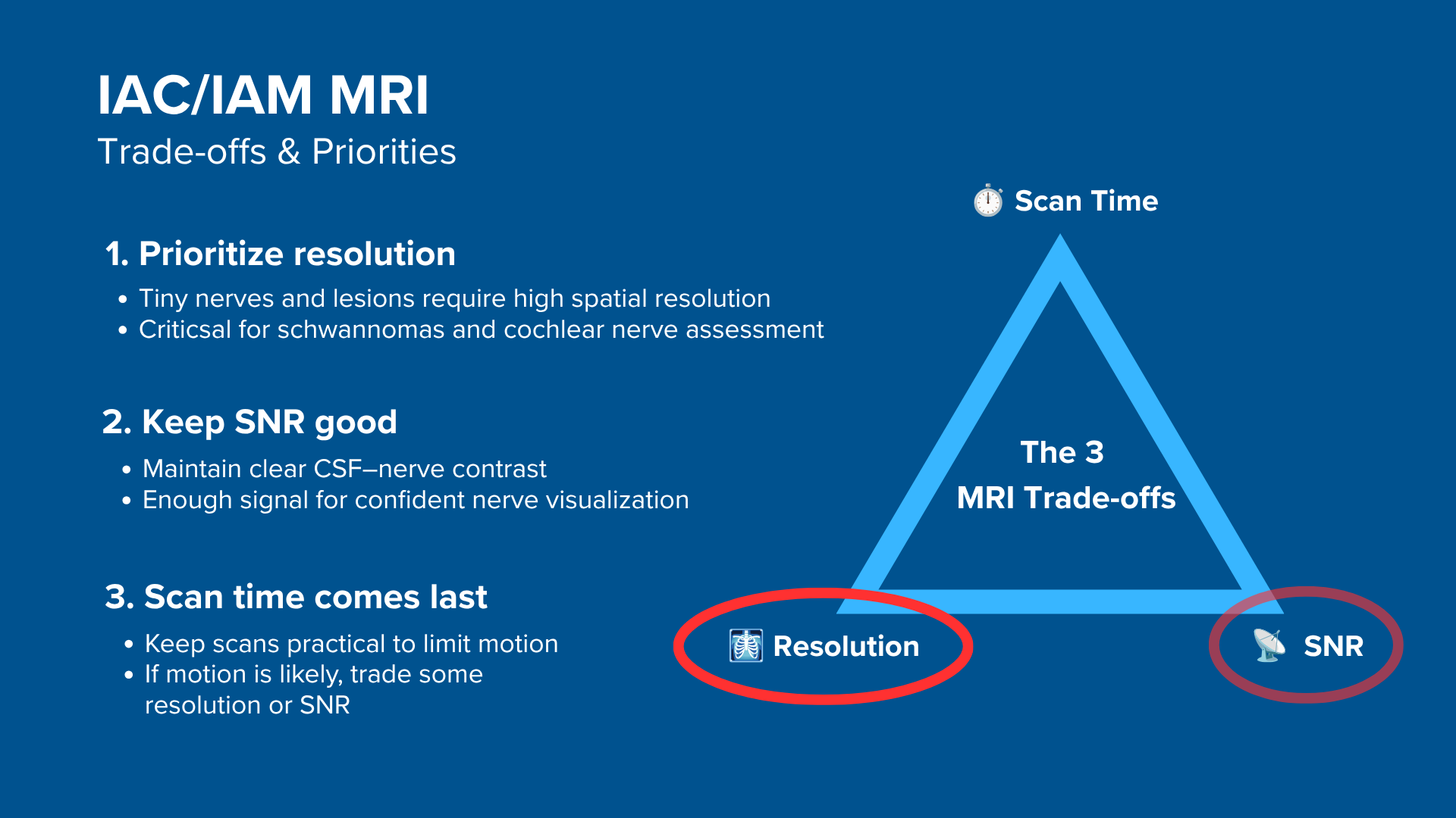
Because the IAC contains millimeter-scale structures, resolution comes first.
We therefore 1) prioritize resolution, 2) maintain enough SNR to keep bright fluid separated from dark nerves, and 3) optimize scan time last. If the patient cannot hold still, time trumps everything.
The two 3D high-resolution sequences do most of the diagnostic work.
3D axial bSSFP (CISS, FIESTA-C) and 3D axial T2 TSE (SPACE, CUBE, VISTA) give isotropic voxels of 1 mm or smaller, plus strong contrast between bright CSF and dark nerves. Tiny filling defects are found here first, then characterized by the 2D thin-slice and post-contrast T1 FS sequences.
Avoid these 5 common IAC/IAM artifacts.
Artifacts
Solution – How to Avoid It
Motion artifacts
Immobilize the patient's head firmly with cushions. Shorten the long 3D sequences using parallel imaging. Clearly tell the patient not to swallow during the important 3D scans.
Banding artifacts
Shim locally over the temporal bones. If bands persist, confirm you are on a phase-cycled variant (CISS or FIESTA-C), or switch to 3D T2 TSE.
Susceptibility artifacts
Switch from gradient-echo sequences (like bSSFP) to fast spin-echo sequences such as 3D T2 TSE. Spin-echo uses refocusing pulses that recover signal lost to magnetic field distortions near air and bone.
Wrap-around (aliasing) artifacts
Turn on phase oversampling (fold-over suppression). IAC scans use a very small field of view for high resolution, so this stops outside parts of the head (nose or back of skull) from folding into the image.
Failed fat suppression
Shim locally over the temporal bones and check the center frequency, since spectral fat sat fails when the fat peak drifts off resonance. Switch to Dixon if suppression still fails near the petrous apex.
Intro to IAC/IAM MRIs
The internal auditory canal (IAC), also called the internal auditory meatus (IAM), is a short bony tunnel inside the petrous part of the temporal bone. It connects the posterior cranial fossa to the inner ear. The canal averages around 8.5 mm in length and roughly 4 mm in diameter, is lined by dura, and is filled with cerebrospinal fluid.
Everything of clinical interest here is small. The cochlea, the vestibule, the semicircular canals, and four separate cranial nerve branches all sit inside a space narrower than a pencil. This is why the IAC/IAM study is one of the most technically demanding protocols in neuro MRI, and why it typically takes 45 to 60 minutes to complete.
The study is usually requested for asymmetric or sudden sensorineural hearing loss, unilateral tinnitus, vertigo, or facial nerve weakness. MRI is the reference standard for these symptoms, because it can show masses as small as 2 mm inside the canal. Vestibular schwannoma is by far the most common finding, accounting for roughly 80% of cerebellopontine angle (CPA) tumors, followed by meningioma at 10 to 15%.
The 4 Nerves Inside the IAC, and Why Their Position Matters
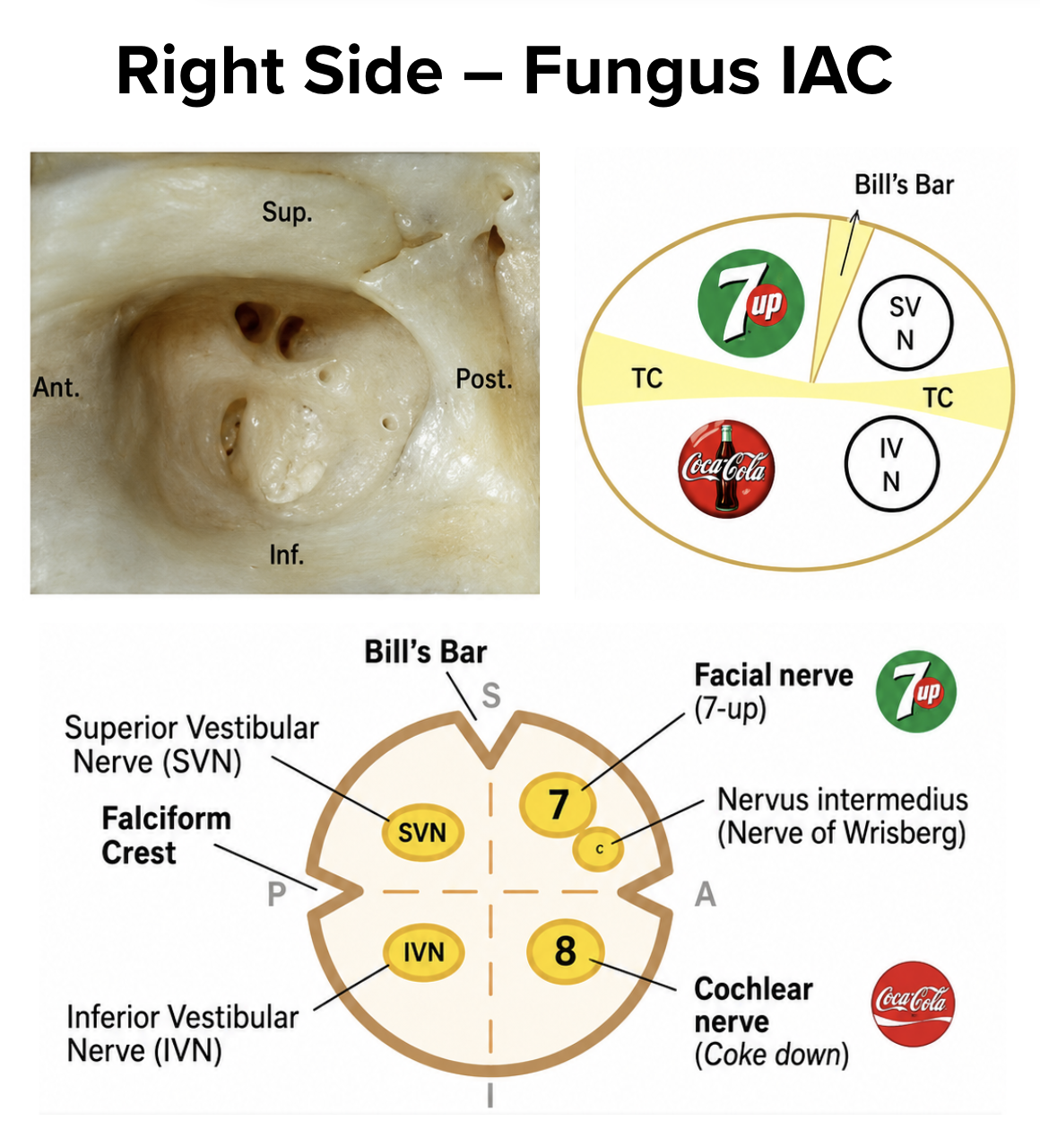
At the lateral end of the canal, the fundus, two thin bony crests divide the space. The transverse crest (also called the falciform crest) splits the canal into a superior and an inferior half. A vertical crest known as Bill’s bar then splits the superior half into an anterior and a posterior part, separating the facial nerve from the superior vestibular nerve. There is no comparable bony crest in the inferior half, where the cochlear nerve simply lies anterior to the inferior vestibular nerve.
Radiologically, the fundus is therefore described as four quadrants, each carrying one nerve:
Anterosuperior: facial nerve (CN VII), together with the nervus intermedius.
A common way to remember the anterior two is “7-Up, Coke down”: the seventh nerve sits superior, the cochlear nerve sits inferior.
Knowing this four-quadrant anatomy matters for two practical reasons.
First, when a schwannoma is found, the radiologist needs to know which nerve it arose from, and that depends on which quadrant it occupies. A facial nerve schwannoma extending into the labyrinthine segment is managed very differently from a vestibulocochlear schwannoma.
Second, in cochlear implant work-up, the question is whether a cochlear nerve is present at all in the anteroinferior quadrant. Both questions can only be answered if your slices are thin enough and angled well enough to resolve the four nerves separately.
The labyrinthine artery also runs through the canal. In a minority of patients, a loop of the anterior inferior cerebellar artery (AICA) enters the canal as well, which is a normal variant.
How to Balance the 3 Trade-offs in IAC/IAM MRIs
In MRI, we always face a trade-off between 3 key metrics:
Scan Time: How fast a pulse sequence can be completed.
Resolution: How much detail the image can display.
SNR: How clear the image is, meaning how much signal we have compared with noise.
Improving one of these metrics often reduces the performance of the others.
To decide what trade-offs to make, we must consider the needs of each clinical situation.
For IAC/IAM MRIs, we face these challenges:
The internal auditory canal and inner ear contain very small structures, including the cochlea, semicircular canals, and the separate branches of cranial nerves VII and VIII. Without high spatial resolution, we may miss small intracanalicular schwannomas or fail to assess cochlear nerve deficiency clearly.
We rely heavily on high-resolution sequences, such as 3D bSSFP and 3D T2 TSE. These sequences use bright CSF or inner-ear fluid to outline darker nerves, vessels, and filling defects. Because higher resolution reduces voxel size and can lower SNR, we need enough SNR to keep this fluid-to-nerve contrast clear.
These high-resolution sequences can take longer to acquire and are vulnerable to motion. Even small head motion or swallowing can blur the fine details we are trying to see.
Therefore, we typically:
Prioritize resolution to clearly visualize tiny cranial nerves, small IAC lesions, and detailed inner-ear anatomy.
Maintain strong enough SNR to preserve the contrast between bright fluid and dark nerves, vessels, or small lesions.
Optimize scan time last, keeping it as short as practical so motion does not reduce the high-resolution detail.
Note! Prioritizing resolution in IAC/IAM MRIs is only a general guideline, NOT a strict rule. If your patient cannot stay still, scan time moves to the top of the list, because a blurred 0.7 mm acquisition is worth less than a sharp 1 mm one. The right balance always depends on your field strength, patient cooperation, and clinical question.
IAC/IAM Health Conditions and the MRI Sequences That Reveal Them
The IAC/IAM MRI study can help us diagnose a wide range of health conditions. The table below lists some of the most common conditions and what pulse sequences reveal them:
Shows tissues and lesions that are already bright before contrast. This helps identify fat, blood products, and cholesterol-rich material. Prevents mistaking natural T1 brightness for true enhancement on post-contrast images.
Fluid, cystic change, and mass effect:
• Large CPA/IAC mass effect
• Brainstem compression
• Cystic CPA lesion / arachnoid cyst
T2 TSE
Highlights water-rich structures like CSF, edema, and simple fluid. This makes cystic lesions and compression easier to assess. Useful for showing the broader CPA, posterior fossa, and brainstem anatomy.
Creates strong contrast between bright CSF and dark nerves, vessels, or small soft-tissue lesions. This makes tiny IAC filling defects easier to spot. Ideal for mapping the relationship between cranial nerves VII/VIII and nearby vessels.
Provides high-resolution imaging of the cochlea, vestibule, semicircular canals, and IAC nerves. Normal inner-ear fluid appears bright. Filling defects, fibrosis, ossification, or an absent/small cochlear nerve become easier to see.
Enhancing tumors and inflammation:
• Vestibular schwannoma
• CPA meningioma
• Active labyrinthitis or facial/vestibulocochlear neuritis
T1 FS TSE (Post-contrast)
Shows abnormal enhancement after gadolinium. Fat suppression removes bright skull-base fat and marrow signal, making enhancing tumors, inflamed nerves, and labyrinthine enhancement stand out more clearly. Coronal images help show dural tails and vertical nerve enhancement.
Do We Always Need Contrast?
Not always. Many centers now screen for vestibular schwannoma with high-resolution 3D T2 imaging alone, with no gadolinium at all. A high-resolution 3D acquisition shows an intracanalicular schwannoma as a dark filling defect against bright CSF, and for tumors inside the canal or the CPA cistern this works well.
The limitation is the labyrinth. Small intralabyrinthine schwannomas and early labyrinthitis sit inside the inner-ear fluid spaces and can be much harder to call on T2 alone, which is the main argument for keeping post-contrast T1 fat-saturated sequences in the protocol.
In practice, this means two things for you at the console:
First, check your local protocol before assuming contrast is given.
Second, if the study is non-contrast, your 3D bSSFP (and 3D T2 TSE, if your protocol includes it) becomes the entire examination, so the quality of these high-resolution 3D sequences is the whole result.
This guide covers the full contrast-enhanced protocol, since it includes every sequence you would run in either version of the study.
How to Perform an IAC/IAM Protocol
The step-by-step guide below will show you how to set up and perform an IAC/IAM MRI protocol in practice.
We will perform the protocol in 3 parts:
Set up the Patient and MRI Scanner
Plan and Acquire the Protocol Sequences
Review the Images
Part 1: Set up the Patient and MRI Scanner
1. Position the Patient in the Scanner
Lay the patient head-first and supine (on their back) with the head centered at the scanner’s isocenter, exactly as for a routine neuro examination.
Motion control is not an optional extra in this protocol. It is part of the acquisition. Pack the head firmly with cushions on both sides, and take the extra minute to make the patient genuinely comfortable, because a comfortable patient moves less over a 45 to 60 minute study.
Tell the patient explicitly not to swallow during the long 3D acquisitions, and warn them before each one starts.
Use an 8-channel conformal coil. Gives enough receive channels for GRAPPA acceleration on these high-resolution sequences, while covering both temporal bones symmetrically for side-to-side comparison.
Once the patient is in place, review your scanner’s hardware settings.
In this guide, we will use the following settings:
Scanner Setting
Value
Why This Value
Magnetic field strength
1.5 T
The most common clinical field strength, giving enough SNR for this protocol with less susceptibility and B1 artifact than 3 T, an advantage that matters near the air and bone interfaces at the skull base.
Maximum gradient strength
45 mT/m
Provides strong, versatile gradient performance that supports fast imaging and precise spatial encoding.
Coil
8-channel conformal coil
Gives enough receive channels for GRAPPA acceleration on these high-resolution sequences, while covering both temporal bones symmetrically for side-to-side comparison.
This hardware setup is widely used in clinical practice. It balances acquisition time, image quality, and patient comfort.
Remember that every parameter in this guide is tied to this hardware setup. Change the field strength, the gradient performance, or the coil and the optimal bandwidth, turbo factor, and acceleration factor all change with it.
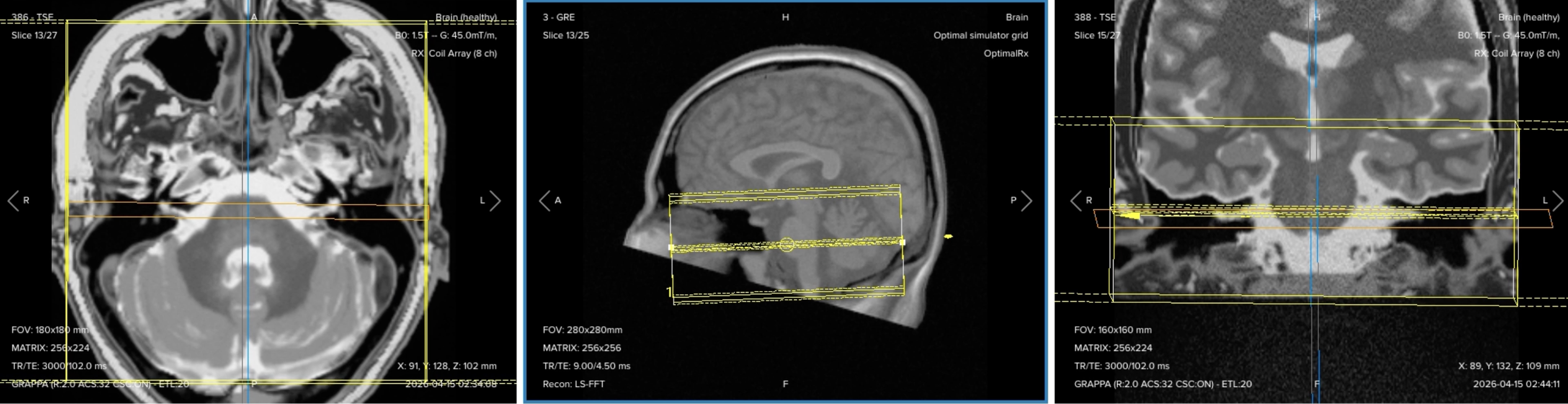
3. Capture the Initial Localizer Images
Before we can perform any MRI protocol, we must always capture initial localizer images of the patient. These images act as a guide for planning the detailed scans we will perform next.
We should always capture localizers in three planes:
Axial
Sagittal
Coronal
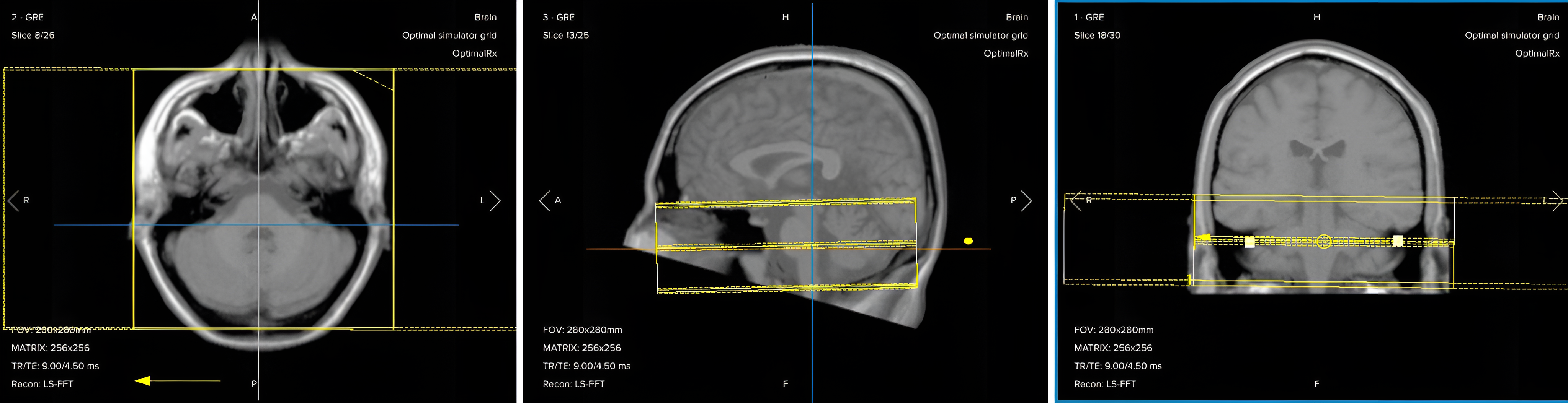
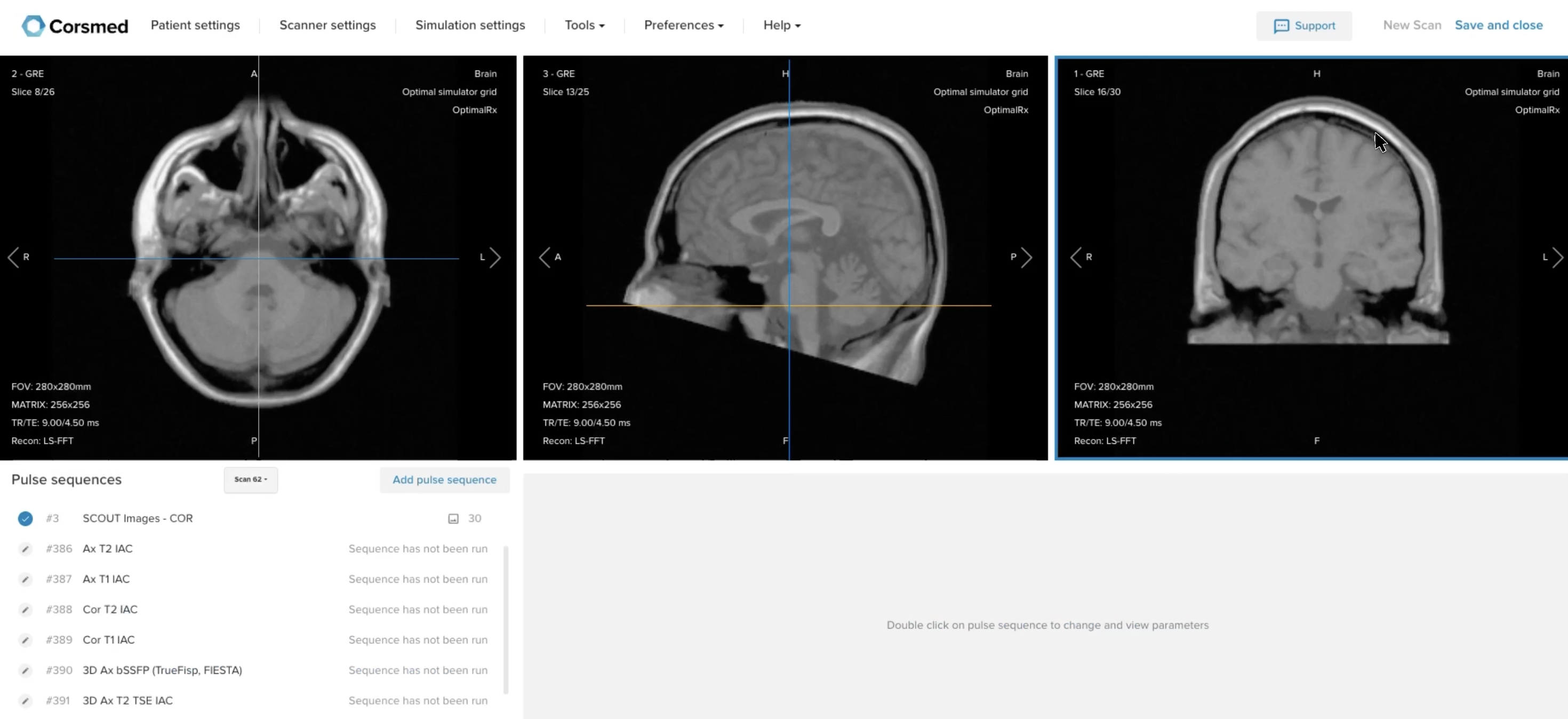
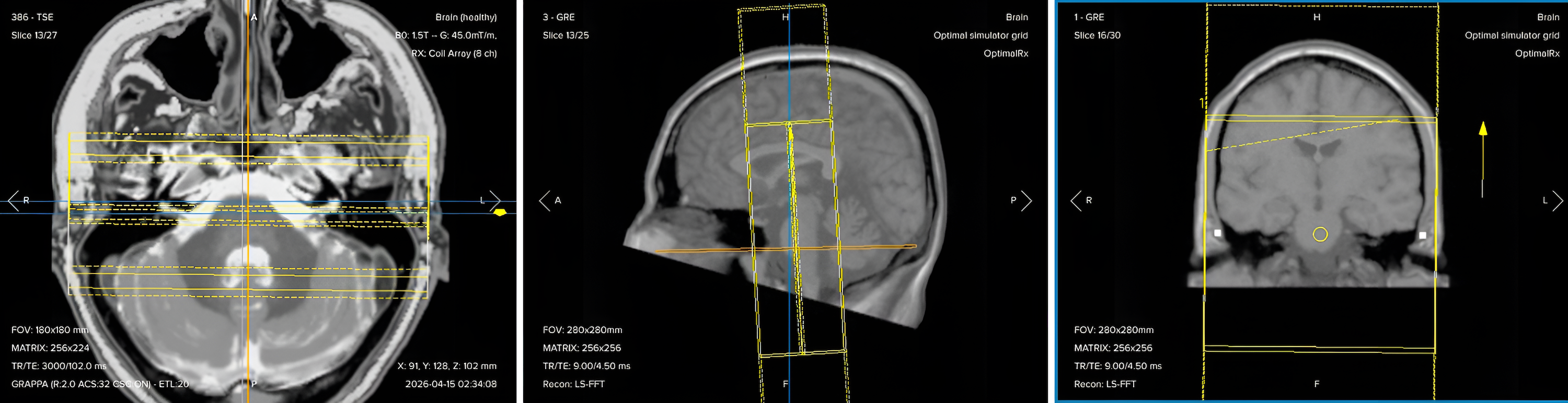
Once acquired, load the initial localizer images into the three viewports and scroll through each stack:
Axial: scroll until both internal auditory canals are clearly visible.
Sagittal: stop on a mid-brain slice, which gives you the brainstem and the other landmarks you need for angulation.
Coronal: stop on a slice that shows the IAC region.
✅ Correct setup of localizer images in the three viewports on the Corsmed MRI simulator:
Part 2: Plan and Acquire the Protocol Sequences
When all preparations are ready, we can start planning and acquiring the protocol sequences.
The 8 Sequences of a Standard IAC/IAM MRI Protocol
Axial T2 TSE (thin slice)
Axial T1 TSE (thin slice)
Coronal T2 TSE (thin slice)
Coronal T1 TSE (thin slice)
3D Axial bSSFP (CISS / FIESTA-C)
3D Axial T2 TSE (SPACE / CUBE / VISTA)
Axial T1 FS TSE (Post-Contrast)
Coronal T1 FS TSE (Post-Contrast)
This protocol pairs two acquisition strategies. The 2D thin-slice sequences in two planes and two contrasts give us tissue characterization and a pre-contrast baseline. The two 3D high-resolution sequences give us the isotropic detail that the diagnosis actually depends on, down to 0.7 mm on the bSSFP.
Keep in mind that this is a comprehensive example protocol, not a fixed standard. The exact sequences vary with the radiological requirements at your institution, and the 3D axial T2 TSE in particular is often an optional add-on rather than a fixed part of the study.
In the sections below, we go through how to plan and set up each sequence.
1. Axial T2 TSE
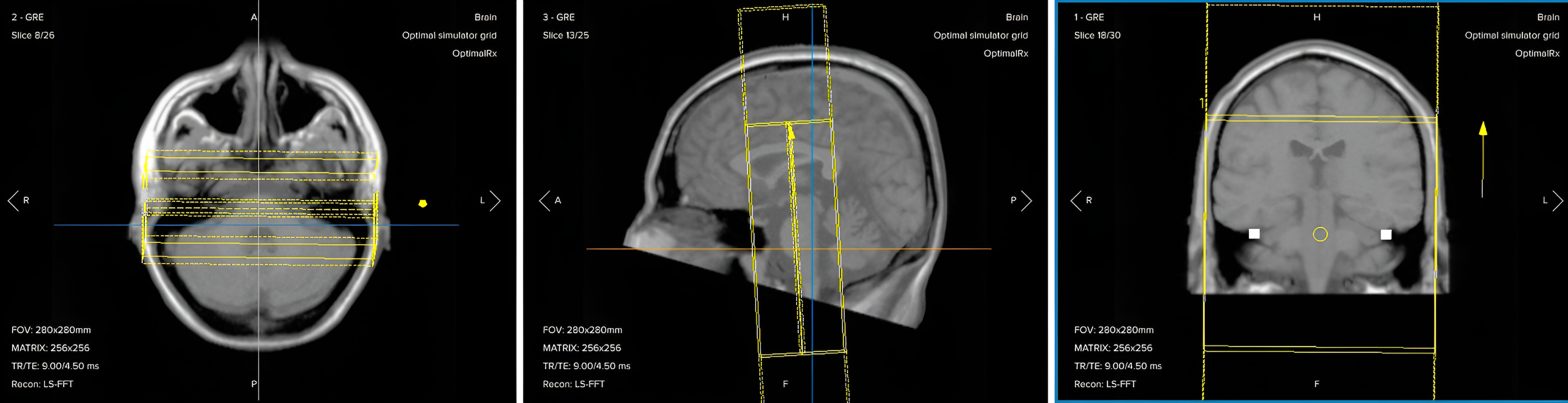
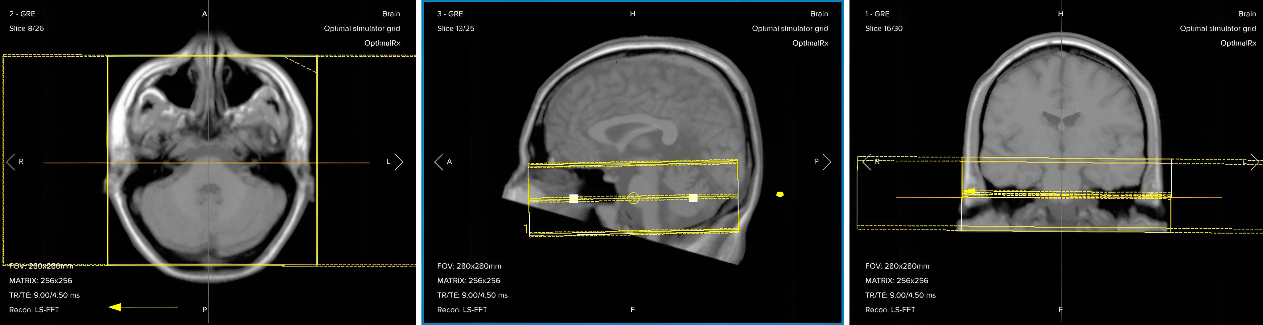
✅ Correct planning:
Planning Instructions:
Use both internal auditory canals as your anatomical reference.
Align the slices as follows:
Axial localizer: Angle the slice as a parallel line that bisects both IAC regions.
Coronal localizer: Fine-tune the angle so the slice cuts symmetrically through the middle of both canals.
Sagittal localizer: Angle the slice package perpendicular to the brainstem.
Add enough slices to cover from the level of the hippocampus superiorly down to the foramen magnum or the C1 vertebral body inferiorly. Use the coronal and sagittal views to confirm both borders.
Keep the field of view tightly focused on the IAC region. The whole point of this sequence is resolution.
Parameters for Axial T2 TSE:
Parameter
Recommended Values
Why These Values
Echo Time (TE)
80–120 ms
Long TE is required for T2 contrast.
Repetition Time (TR)
3,000–5,000 ms
Long TR is required for T2 contrast.
Field of View (FOV)
180 × 180 mm
Small FOV gives a zoomed-in view of the IAC region.
Matrix
256 × 224
Medium matrix that delivers 0.7 × 0.8 mm in-plane resolution at this FOV.
Number of Slices
25–30
Enough slices to fully cover from the hippocampus down to the foramen magnum.
Slice Thickness
2 mm
Thin enough to resolve the four nerve branches inside a canal roughly 4 mm across, at some cost in SNR.
Slice Gap
0.2 mm
10% of slice thickness, which limits cross-talk without hiding anatomy.
NEX / Averages
2
To get enough SNR, while keeping scan time short.
Bandwidth per pixel
220–250 Hz/px
Set close to the 220 Hz fat-water offset at 1.5T, which holds fat-water misregistration to about one pixel while preserving SNR.
Turbo Factor / ETL
15–20
Higher turbo factor reduces scan time, and long effective TE provides T2 weighting.
Parallel Imaging
GRAPPA, acceleration factor 2
Halves the phase-encoding steps to keep scan time down, at a modest SNR cost.
Fold-over Suppression
Yes
Prevents wrap-around from the nose and posterior skull folding into the small FOV.
Fat Suppression
None
Not needed for this sequence.
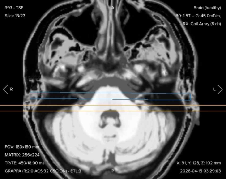
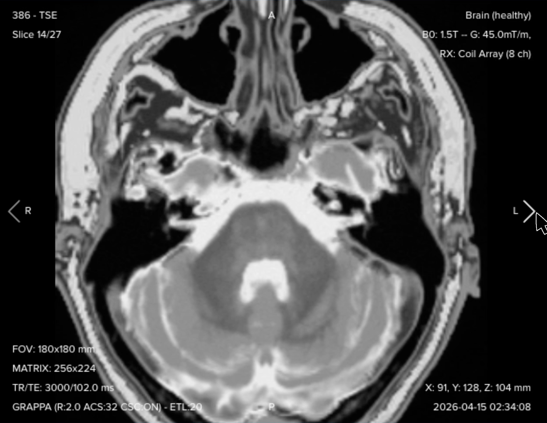
Resulting axial T2 image, scrolled to the IAC region:
Scroll down to the IAC region and check the result. The cranial nerves should be clearly outlined against bright cerebrospinal fluid, with no motion blur and no wrap.
2. Axial T1 TSE
✅ Correct planning:
Planning Instructions:
This sequence must be an identical copy of the axial T2 in terms of geometry.
Open the sequence, right-click on the axial T2, and copy all of the slices.
Identical alignment is what makes the two contrasts comparable to the radiologist. Do not re-plan by hand.
Parameters for Axial T1 TSE:
Parameter
Recommended Values
Why These Values
Echo Time (TE)
10–20 ms
Short TE is required for T1 contrast.
Repetition Time (TR)
400–700 ms
Short TR is required for T1 contrast.
Field of View (FOV)
180 × 180 mm
Copied from the axial T2 to keep geometry identical.
Matrix
256 × 224
Copied from the axial T2.
Number of Slices
25–30
Copied from the axial T2.
Slice Thickness
2 mm
Copied from the axial T2.
Slice Gap
0.2 mm
Copied from the axial T2.
NEX / Averages
2
To get enough SNR, while keeping scan time short.
Bandwidth per pixel
220–250 Hz/px
Holds fat-water misregistration to about one pixel at 1.5T.
Turbo Factor / ETL
3
Kept short so the effective TE stays short, preserving T1-weighting.
Parallel Imaging
GRAPPA, acceleration factor 2
Same acceleration as the axial T2.
Fold-over Suppression
Yes
Prevents wrap-around artifacts.
Fat Suppression
None
Fat must stay bright here, so it can act as the pre-contrast reference.
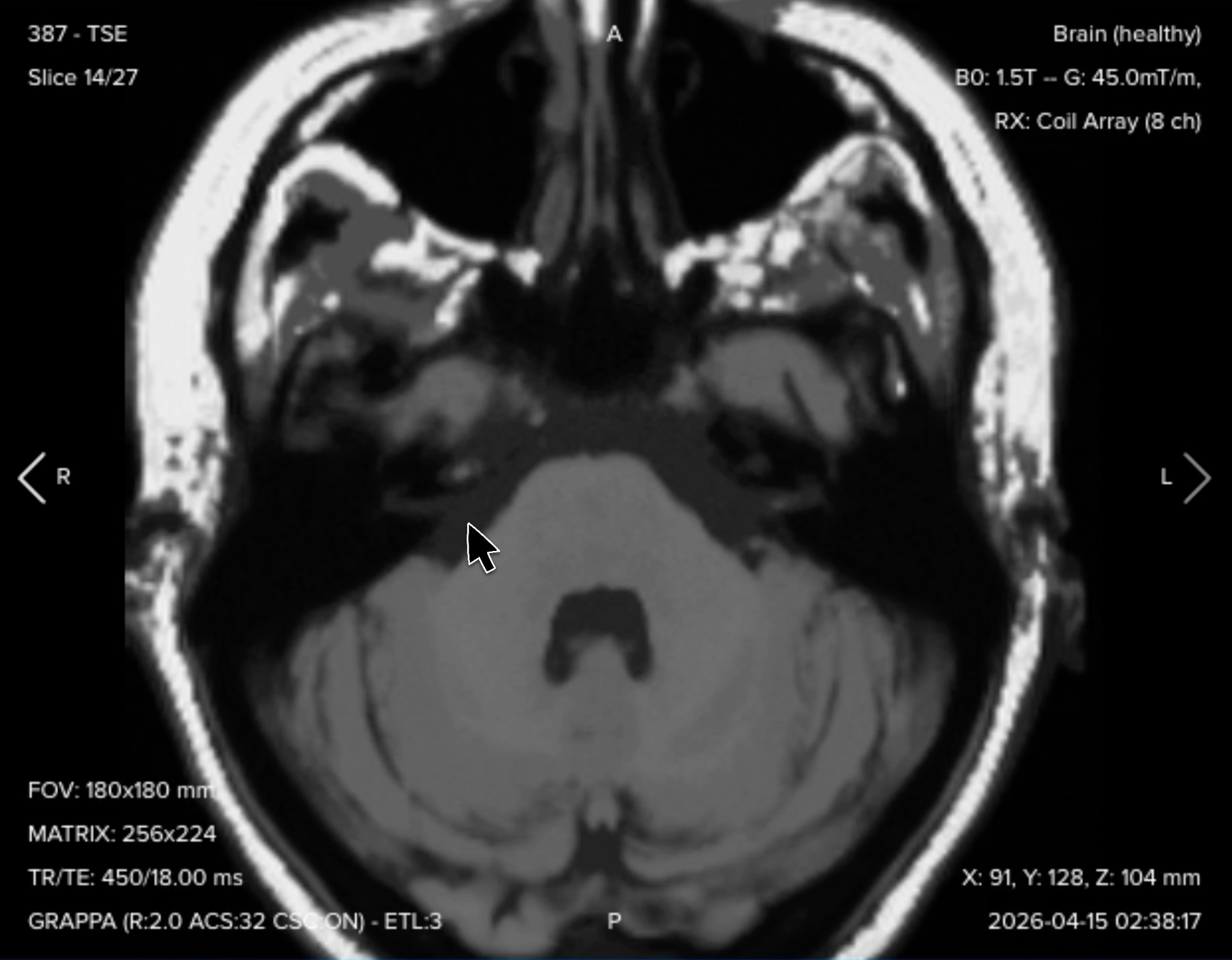
Resulting axial T1 image:
This axial T1 establishes the baseline anatomy. Without it, the radiologist cannot tell a genuinely enhancing lesion from something that was already bright on T1, such as a lipoma or a cholesterol granuloma.
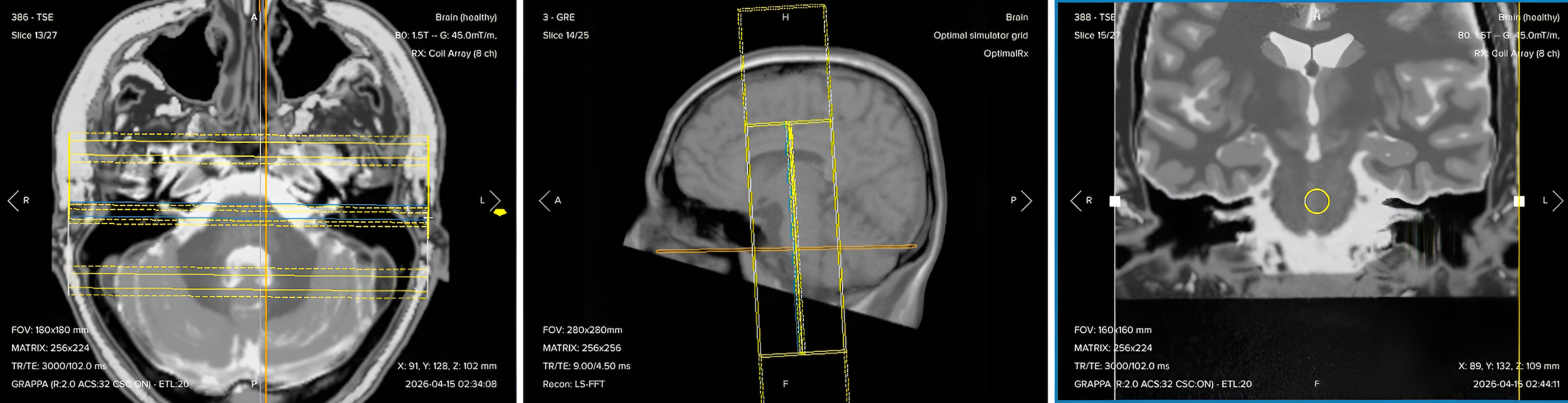
3. Coronal T2 TSE
✅ Correct planning:
Planning Instructions:
Plan this sequence from the high-resolution axial T2 you just acquired, not from the localizer.
Scroll to the IAC region on the axial images, right-click, and set the perpendicular position to create the coronal.
Align the slices as follows:
Axial T2: Angle the slices to run parallel to both IAC structures. This is the most important angulation in the coronal view.
Sagittal localizer: Angle the slices parallel to the brainstem. Shift the slice position onto the brainstem and confirm the slices follow its angle exactly.
Add enough slices to cover from the posterior border of the sphenoid sinuses to the fourth ventricle, which is typically 25 to 30 slices.
Parameters for Coronal T2 TSE:
Parameter
Recommended Values
Why These Values
Echo Time (TE)
80–120 ms
Long TE is required for T2 contrast.
Repetition Time (TR)
3,000–5,000 ms
Long TR is required for T2 contrast.
Field of View (FOV)
160 × 160 mm
Covers both temporal bones, with less in-plane extent needed than on the axial.
Matrix
256 × 224
Delivers 0.6 × 0.7 mm in-plane resolution at this FOV.
Number of Slices
25–30
Enough to cover from the posterior sphenoid sinuses to the fourth ventricle.
Slice Thickness
2 mm
Thin enough to resolve the four nerve branches inside a canal roughly 4 mm across, at some cost in SNR.
Slice Gap
0.2 mm
10% of slice thickness, which limits cross-talk without hiding anatomy.
NEX / Averages
2
To get enough SNR, while keeping scan time short.
Bandwidth per pixel
220–250 Hz/px
Holds fat-water misregistration to about one pixel at 1.5T.
Turbo Factor / ETL
15–20
Higher turbo factor reduces scan time, and long effective TE provides T2 weighting.
Parallel Imaging
GRAPPA, acceleration factor 2
Halves the phase-encoding steps to keep scan time down, at a modest SNR cost.
Fold-over Suppression
Yes
Prevents wrap-around artifacts.
Fat Suppression
None
Not needed for this sequence.
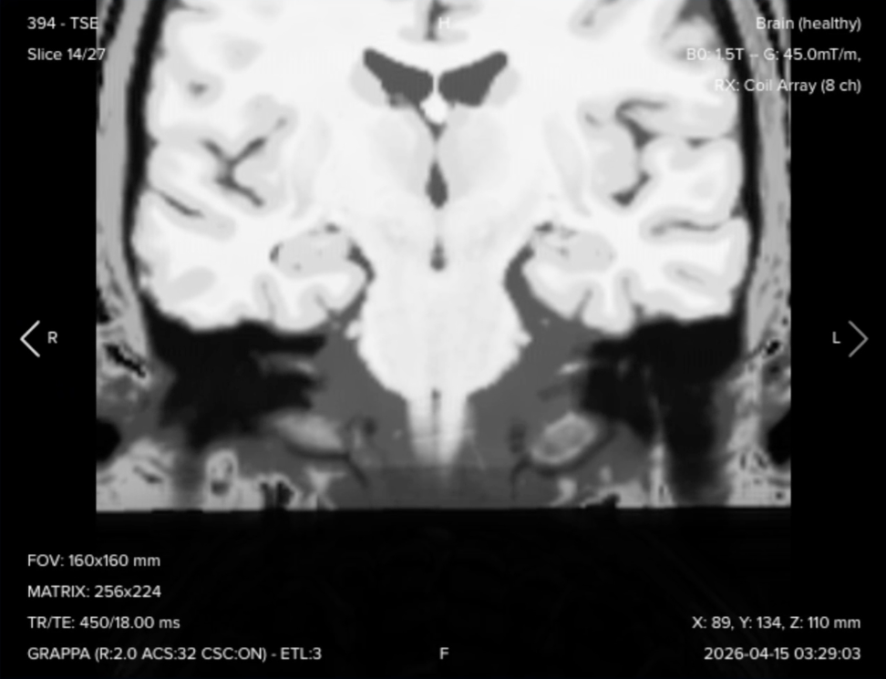
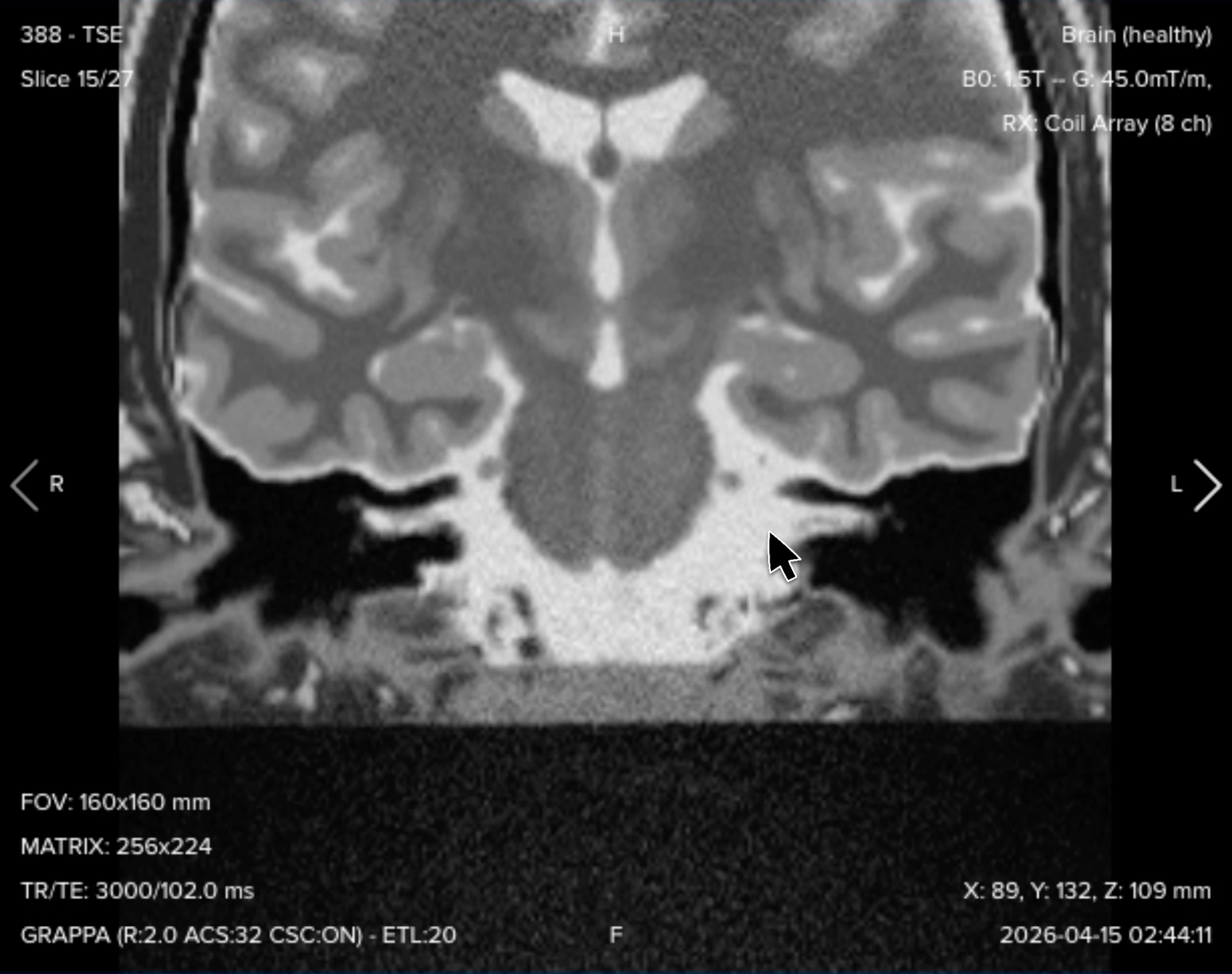
Resulting coronal T2 image:
The coronal view gives a complementary perspective on the cerebellopontine angle (CPA), which helps considerably with lesion detection and with judging how far a lesion extends.
4. Coronal T1 TSE
✅ Correct planning:
Planning Instructions:
Copy the slices directly from the coronal T2 to guarantee an identical position.
Keep the same geometry parameters so the two contrasts can be compared slice for slice.
Parameters for Coronal T1 TSE:
Parameter
Recommended Values
Why These Values
Echo Time (TE)
10–20 ms
Short TE is required for T1 contrast.
Repetition Time (TR)
400–700 ms
Short TR is required for T1 contrast.
Field of View (FOV)
160 × 160 mm
Copied from the coronal T2.
Matrix
256 × 224
Copied from the coronal T2.
Number of Slices
25–30
Copied from the coronal T2.
Slice Thickness
2 mm
Copied from the coronal T2.
Slice Gap
0.2 mm
Copied from the coronal T2.
NEX / Averages
2
To get enough SNR, while keeping scan time short.
Bandwidth per pixel
220–250 Hz/px
Holds fat-water misregistration to about one pixel at 1.5T.
Turbo Factor / ETL
3
Kept short so the effective TE stays short, preserving T1-weighting.
Parallel Imaging
GRAPPA, acceleration factor 2
Same acceleration as the coronal T2.
Fold-over Suppression
Yes
Prevents wrap-around artifacts.
Fat Suppression
None
Fat must stay bright as the pre-contrast reference.
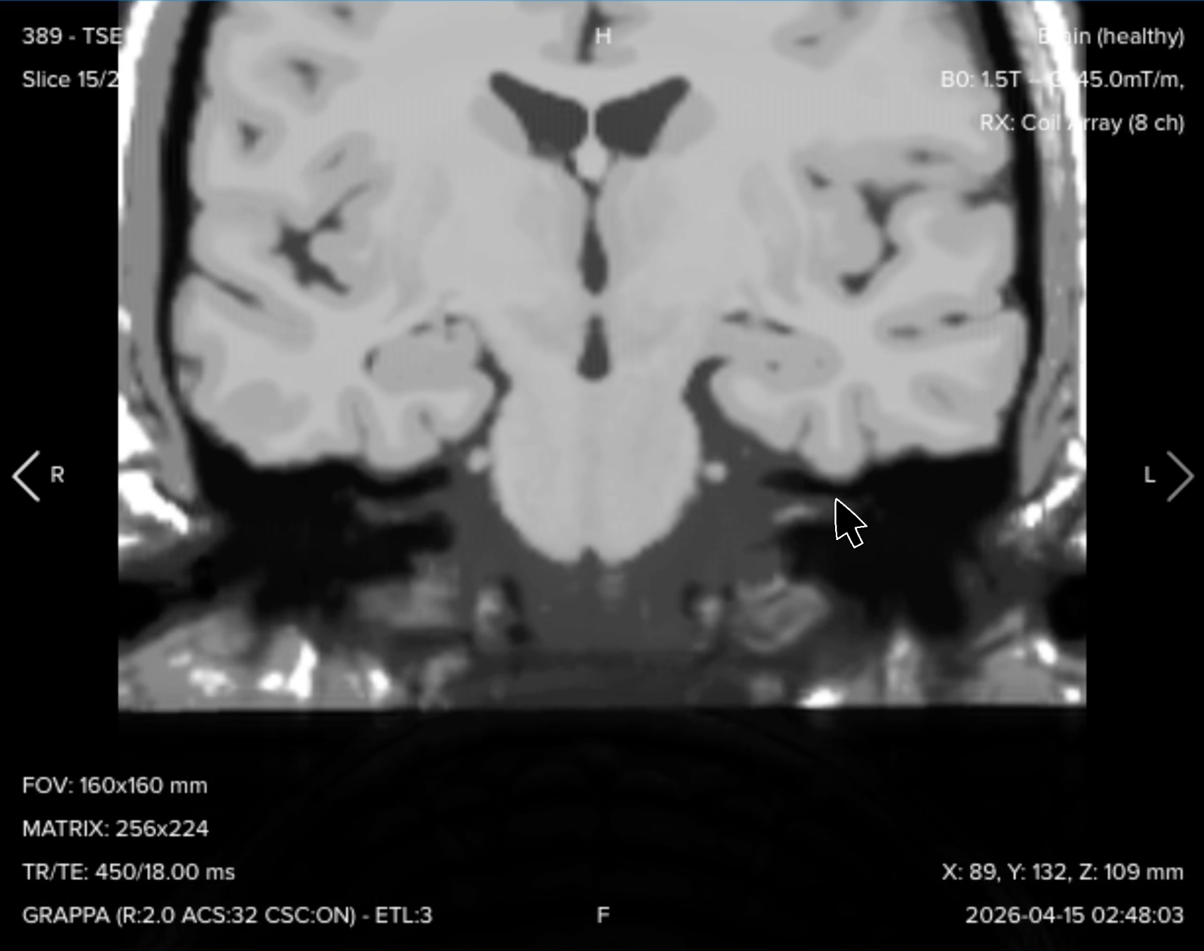
Resulting coronal T1 image:
Tip: In the Corsmed simulator, you can adjust image brightness by holding Ctrl + Alt (Option) and using the up and down arrow keys.
5. 3D Axial bSSFP (CISS / FIESTA-C)
Vendor naming matters here. CISS (Siemens) and FIESTA-C (GE) are dual acquisition, phase-cycled versions of balanced SSFP, and the second phase cycle is what suppresses banding at the skull base. Single acquisition balanced SSFP, sold as TrueFISP or FIESTA, will work but is more prone to banding across the canal.
This is the most important sequence in the protocol. It allows an even thinner slice thickness than the 2D sequences, which is what makes tiny intracanalicular lesions visible at all.
✅ Correct planning:
Planning Instructions:
Plan from your high-resolution coronal T2, not from the localizer. When you have high-resolution images available, always use them to plan the next sequence.
Scroll the coronal T2 to the IAC region and confirm the slice package runs parallel to both canals.
Align the slice to symmetrically bisect both IACs, in the same way as the other axial sequences.
Add enough slices to cover from the hippocampus down to the foramen magnum or the C1 vertebral body. Use 80–90 slices to be certain nothing is missed.
Aim for isotropic resolution, so the dataset supports proper multiplanar reconstruction.
Note that with fold-over suppression active, the field of view will visibly extend beyond the head on the axial plane. This is expected and is what prevents wrap.
Parameters for 3D Axial bSSFP:
Parameter
Recommended Values
Why These Values
Echo Time (TE)
Half of TR (1.8–2.3 ms)
Placed at half the TR so the echo sits symmetrically in the repetition interval; the balance itself comes from gradient moments canceling over each TR.
Repetition Time (TR)
3.5–4.5 ms
Very short TR is inherent to balanced steady-state acquisition.
Flip Angle
60°
Optimized to maximize CSF-to-nerve contrast while avoiding flow artifacts.
Field of View (FOV)
160 × 160 mm
Small FOV focused tightly on the IAC region.
Matrix
230 × 230
Gives 0.7 mm in-plane resolution at this FOV, matching the slice thickness.
Number of Slices
80–90
Enough to cover from the hippocampus down to the foramen magnum. Adjust to the patient's anatomy.
Slice Thickness
0.7 mm
Gives 0.7 mm cubic voxels, which is what makes multiplanar reconstruction usable.
Foldover Direction (Phase)
Right-to-Left (RL)
Reduces flow artifacts across the region of interest.
NEX / Averages
2
Extra average is needed for adequate signal at this voxel size.
Bandwidth per pixel
400–500 Hz/px
Gives a ~2.3 ms readout, short enough to fit inside the 3.5–4.5 ms TR.
Parallel Imaging
GRAPPA, acceleration factor 2
Halves the phase-encoding steps to keep scan time down, at a modest SNR cost.
Fold-over Suppression
Yes
Required. The small FOV would otherwise wrap the nose and posterior skull into the image.
Fat Suppression
None
Not used for this sequence.
Resulting 3D axial bSSFP image at the level of the IAC:
Scroll through the stack. Cranial nerves VII and VIII should appear as sharply defined dark structures inside bright cerebrospinal fluid, with the surrounding brainstem structures clearly resolved.
6. 3D Axial T2 TSE (SPACE / CUBE / VISTA)
This sequence is not always part of a standard protocol. It may be included as an optional add-on depending on your radiologist’s decision.
It serves the same purpose as the 3D bSSFP, but it is far more robust against magnetic susceptibility and flow artifacts, because spin-echo uses refocusing pulses that recover signal lost near air and bone interfaces. At the skull base, that difference matters.
✅ Correct planning:
Planning Instructions:
Bring back the coronal T2 and scroll through to the IAC region.
Confirm the slices are correctly aligned to both canals, using the same angulation and planning as the 3D bSSFP.
Set enough slices to cover from the hippocampus down to the C1 vertebral body or foramen magnum.
Set the fold-over direction to right-left, which helps avoid flow artifacts.
Parameters for 3D Axial T2 TSE:
Parameter
Recommended Values
Why These Values
Effective Echo Time (TE)
100–150 ms
Long effective TE gives the heavy T2 weighting that makes inner-ear fluid bright.
Repetition Time (TR)
1,800–2,000 ms
Long TR required for T2 contrast in a 3D spin-echo acquisition.
Field of View (FOV)
160 × 160 mm
Matched to the 3D bSSFP so the two can be compared directly.
Matrix
160 × 160
Gives 1 mm in-plane resolution at this FOV, matching the slice thickness.
Number of Slices
65–75
Enough to cover from the hippocampus down to C1, with a slightly longer slab than the bSSFP.
Slice Thickness
1 mm
Isotropic 1 × 1 × 1 mm, half the thickness of the 2D acquisitions.
Foldover Direction (Phase)
Right-to-Left (RL)
Reduces flow artifacts across the region of interest.
NEX / Averages
1
A single average keeps scan time down, since this sequence takes longer to acquire than the 3D bSSFP.
Bandwidth per pixel
700–800 Hz/px
Gives a ~1.3 ms readout, which keeps echo spacing short across the long echo train and limits T2 blurring.
Turbo Factor / ETL
70
With 160 phase encodes and GRAPPA 2, this is close to one echo train per partition.
Parallel Imaging
GRAPPA, acceleration factor 2
Halves the phase-encoding steps to keep scan time down, at a modest SNR cost.
Fold-over Suppression
Yes
Prevents wrap-around artifacts.
Fat Suppression
None
Not used for this sequence.
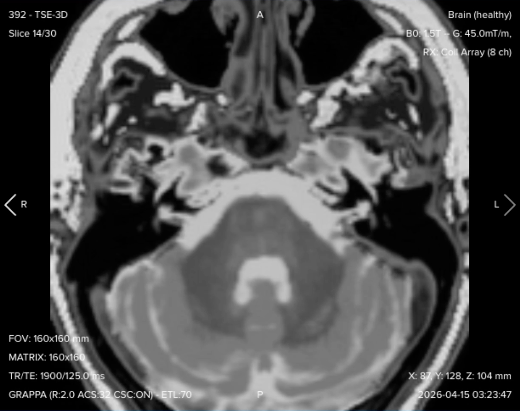
Resulting 3D axial T2 TSE image:
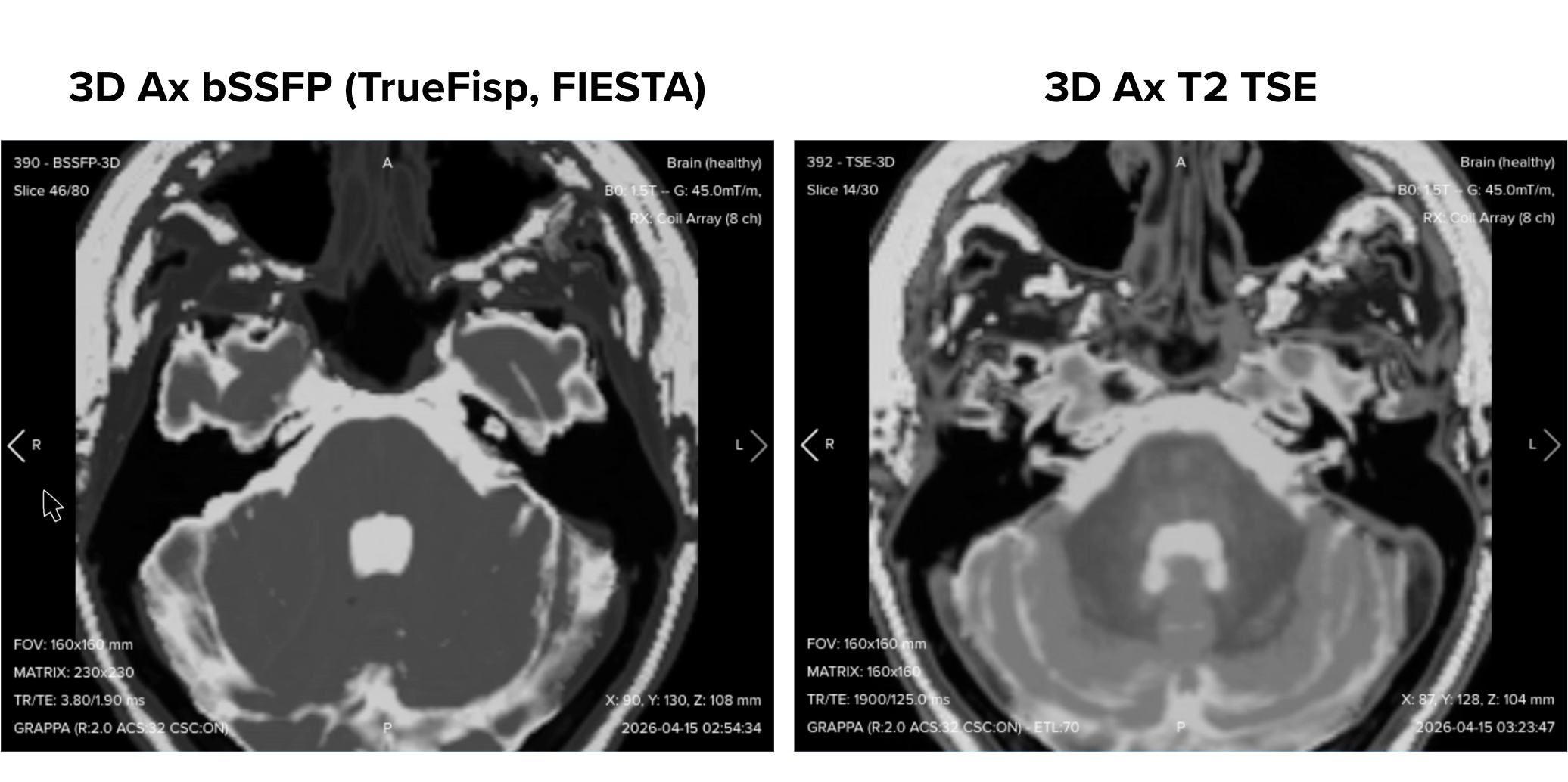
Place the two 3D sequences side by side at the same slice level. Both highlight cerebrospinal fluid, but they earn their place differently. The bSSFP gives the finer voxels and the strongest CSF-to-nerve contrast, while the 3D T2 TSE holds up better at the petrous apex where susceptibility degrades the bSSFP. Comparing them at the same slice level is the fastest way to see that difference.
Side-by-side comparison of the 3D bSSFP and the 3D T2 TSE at the same slice level:
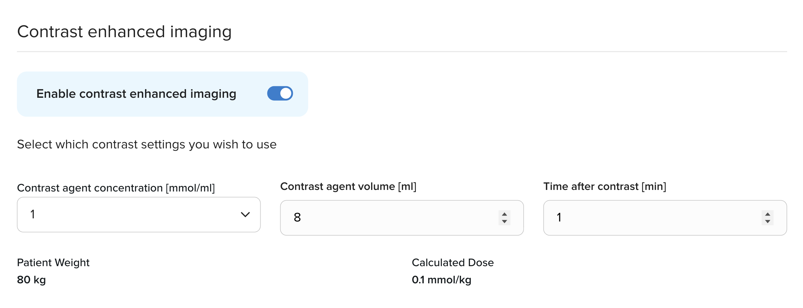
Setting Up the Contrast Injection
Before running the post-contrast sequences, set up the injection.
The volume of contrast agent is set by the patient’s weight. The standard dose is 0.1 mmol/kg. For an 80 kg patient using a 1.0 molar agent such as gadobutrol, that is 8 mL in total.
If your department uses a 0.5 molar agent, the same 0.1 mmol/kg dose requires double the volume, so 16 mL for the same patient. Always check the concentration of the agent in front of you before calculating.
In this protocol, we start acquiring 1 minute after the injection.
Copy the slice geometry and planning from the pre-contrast axial T1 sequence.
Keep the same slice angulation, coverage, and positioning to ensure images of different contrasts can be clearly compared.
Parameters for Axial T1 FS TSE (Post-Contrast):
Parameter
Recommended Values
Why These Values
Echo Time (TE)
10–20 ms
Identical to the pre-contrast axial T1.
Repetition Time (TR)
400–700 ms
Identical to the pre-contrast axial T1.
Field-of-View (FOV)
180 × 180 mm
Copied from the pre-contrast axial T1.
Matrix
256 × 224
Copied from the pre-contrast axial T1.
Number of Slices
25–30
Copied from the pre-contrast axial T1.
Slice Thickness
2 mm
Copied from the pre-contrast axial T1.
Slice Gap
0.2 mm
Copied from the pre-contrast axial T1.
NEX / Averages
2
Maintains signal after the fat-suppression penalty.
Bandwidth per pixel
220–250 Hz/px
Copied from the pre-contrast T1, since fat suppression is the only intended difference.
Turbo Factor / ETL
3
Kept short so the effective TE stays short, preserving T1-weighting.
Parallel Imaging
GRAPPA, acceleration factor 2
Same acceleration as the pre-contrast T1.
Fold-over Suppression
Yes
Prevents wrap-around artifacts.
Fat Suppression
Spectral
Removes bright skull-base fat so enhancing tumors and inflamed nerves stand out.
Resulting post-contrast axial T1 FS image:
Fat should be uniformly dark across the skull base, with any enhancing structure standing out clearly against it. Check this against the pre-contrast axial T1 at the same slice position before moving on.
8. Coronal T1 FS TSE (Post-Contrast)
✅ Correct planning:
Planning Instructions:
Select the pre-contrast coronal T1, copy all slices, and keep the same coverage and planning.
Apply spectral fat suppression.
Confirm the echo time and repetition time are still suitable for T1 weighting.
Parameters for Coronal T1 FS TSE (Post-Contrast):
Parameter
Recommended Values
Why These Values
Echo Time (TE)
10–20 ms
Identical to the pre-contrast coronal T1.
Repetition Time (TR)
400–700 ms
Identical to the pre-contrast coronal T1.
Field-of-View (FOV)
160 × 160 mm
Copied from the pre-contrast coronal T1.
Matrix
256 × 224
Copied from the pre-contrast coronal T1.
Number of Slices
25–30
Copied from the pre-contrast coronal T1.
Slice Thickness
2 mm
Copied from the pre-contrast coronal T1.
Slice Gap
0.2 mm
Copied from the pre-contrast coronal T1.
NEX / Averages
2
Maintains signal after the fat-suppression penalty.
Bandwidth per pixel
220–250 Hz/px
Copied from the pre-contrast T1, since fat suppression is the only intended difference.
Turbo Factor / ETL
3
Kept short so the effective TE stays short, preserving T1-weighting.
Parallel Imaging
GRAPPA, acceleration factor 2
Same acceleration as the pre-contrast T1.
Fold-over Suppression
Yes
Prevents wrap-around artifacts.
Fat Suppression
Spectral
Removes bright skull-base fat so enhancing tumors and inflamed nerves stand out.
Resulting post-contrast coronal T1 FS image:
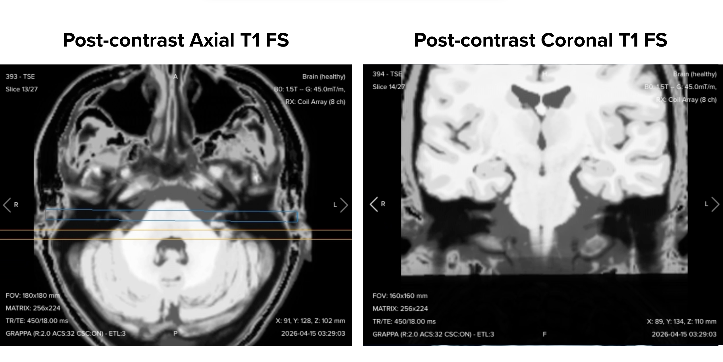
Place this alongside the post-contrast axial from the previous step. Together they give the two planes needed to confirm enhancement and describe how far it extends.
How to Avoid Artifacts When Planning the Sequences
The table below lists the 5 common IAC/IAM artifacts, and what techniques you can use to avoid them:
Artifacts
Solution – How to Avoid It
Motion artifacts
Immobilize the patient's head firmly with cushions. Shorten the long 3D sequences using parallel imaging. Clearly tell the patient not to swallow during the important 3D scans.
Banding artifacts
Shim locally over the temporal bones. If bands persist, confirm you are on a phase-cycled variant (CISS or FIESTA-C), or switch to 3D T2 TSE.
Susceptibility artifacts
Switch from gradient-echo sequences (like bSSFP) to fast spin-echo sequences such as 3D T2 TSE. Spin-echo uses refocusing pulses that recover signal lost to magnetic field distortions near air and bone.
Wrap-around (aliasing) artifacts
Turn on phase oversampling (fold-over suppression). IAC scans use a very small field of view for high resolution, so this stops outside parts of the head (nose or back of skull) from folding into the image.
Failed fat suppression
Shim locally over the temporal bones and check the center frequency, since spectral fat sat fails when the fat peak drifts off resonance. Switch to Dixon if suppression still fails near the petrous apex.
Part 3: Review the Images
Finally, we will review the images to ensure all the anatomical information we need is clear.
These key structures must be clearly visible in an IAC/IAM MRI:
Cranial nerves VII and VIII within the canal, ideally resolved as separate branches
The porus acusticus and the fundus
Cochlea, vestibule, and all three semicircular canals
Cerebellopontine angle cistern and its CSF spaces
Brainstem and the fourth ventricle
Petrous apex and skull-base marrow
AICA and its relationship to cranial nerves VII and VIII
Below, we will go through all the different image contrasts and explain their specific role in imaging the IAC/IAM.
T2 TSE – Fluid, Cystic Change, and Mass Effect
T2-weighted imaging makes fluids appear bright. This contrast is ideal for tissues and abnormalities with high water content.
In IAC/IAM MRI, the 2D T2 sequences show the broader CPA, posterior fossa, and brainstem anatomy, which is what you need to assess large masses, brainstem compression, and arachnoid cysts.
✅ Axial T2 TSE of the IAC, correct image example:
Things to look for in Axial T2:
Cranial nerves clearly outlined as dark structures against bright CSF.
Symmetry between the two canals.
No mass effect on the brainstem or the fourth ventricle.
Sharp detail with no motion blur.
✅ Coronal T2 TSE of the IAC and cerebellopontine angle, correct image example:
Things to look for in Coronal T2:
Complementary view of the cerebellopontine angle.
Vertical extent of any lesion, from the canal into the CPA cistern.
Coverage from the posterior sphenoid sinuses back to the fourth ventricle.
T1 TSE – Baseline Anatomy and T1-Bright Mimics
T1-weighted imaging makes fat appear bright and fluid dark. This contrast is ideal for fat-rich tissues and structural abnormalities.
In IAC/IAM MRI, the pre-contrast T1 sequences do one job that nothing else can do: they show what was already bright before any contrast was given. Lipomas, labyrinthine hemorrhage, and cholesterol granulomas are all intrinsically T1-bright, and without this baseline they can be mistaken for enhancement.
✅ Axial T1 TSE of the IAC, correct image example:
Things to look for in Axial T1:
Clean T1 contrast with good angulation through the canals.
Any intrinsically bright material inside the canal, the labyrinth, or the petrous apex.
Bright subcutaneous fat, which is your reference for the post-contrast comparison.
No artifacts across the IAC region.
✅ Coronal T1 TSE of the IAC, correct image example:
Things to look for in Coronal T1:
Anatomical detail in a plane that complements the axial views.
Confirmation of findings seen on the axial T1.
How far any lesion extends in the superior-inferior direction.
3D bSSFP – The Highest-Detail View of the Nerves
3D balanced steady-state free precession, known as CISS or FIESTA-C in its phase-cycled form, produces the strongest available contrast between bright CSF and dark nerves at sub-millimeter isotropic resolution.
This is where tiny intracanalicular vestibular schwannomas, AICA loops, and vascular contact with cranial nerves VII and VIII are detected.
✅ 3D axial bSSFP of the IAC, correct image example showing cranial nerves against bright CSF:
Things to look for in 3D bSSFP:
All four nerve branches resolved separately where the anatomy allows.
Any filling defect inside the CSF column of the canal.
The course of AICA and whether it contacts or loops around the nerves.
No dark banding across the canal, which would indicate a shimming problem.
3D T2 TSE – Inner-Ear Fluid and the Cochlear Nerve
3D T2 turbo spin echo, known as SPACE, CUBE, or VISTA, delivers 1 mm isotropic resolution, slightly coarser than the bSSFP, with far greater robustness near air and bone interfaces.
It is the sequence of choice for inner-ear fluid assessment: intralabyrinthine schwannomas, cochlear fibrosis, labyrinthitis ossificans, and cochlear nerve aplasia or hypoplasia.
✅ 3D axial T2 TSE of the IAC and inner ear, correct image example:
Things to look for in 3D T2 TSE:
Bright, uniform fluid signal throughout the cochlea, vestibule, and semicircular canals.
Any filling defect or loss of the normal fluid signal inside the labyrinth.
A cochlear nerve of normal caliber in the anteroinferior quadrant.
Clean anatomy at the petrous apex, where bSSFP is most vulnerable to susceptibility.
T1 FS TSE Post-Contrast – Enhancing Tumors and Inflammation
Post-contrast T1 with fat suppression shows abnormal enhancement after gadolinium. Removing the bright skull-base fat and marrow signal is what makes enhancing tumors, inflamed nerves, and labyrinthine enhancement stand out.
Post-contrast axial and coronal T1 fat-suppressed images of the IAC side by side:
Things to look for in Post-Contrast T1 FS:
Uniform, complete fat suppression across the whole skull base.
Any enhancement within the canal, along the nerves, or inside the labyrinth.
A dural tail, which points toward meningioma rather than schwannoma.
Identical slice positions to the pre-contrast series.
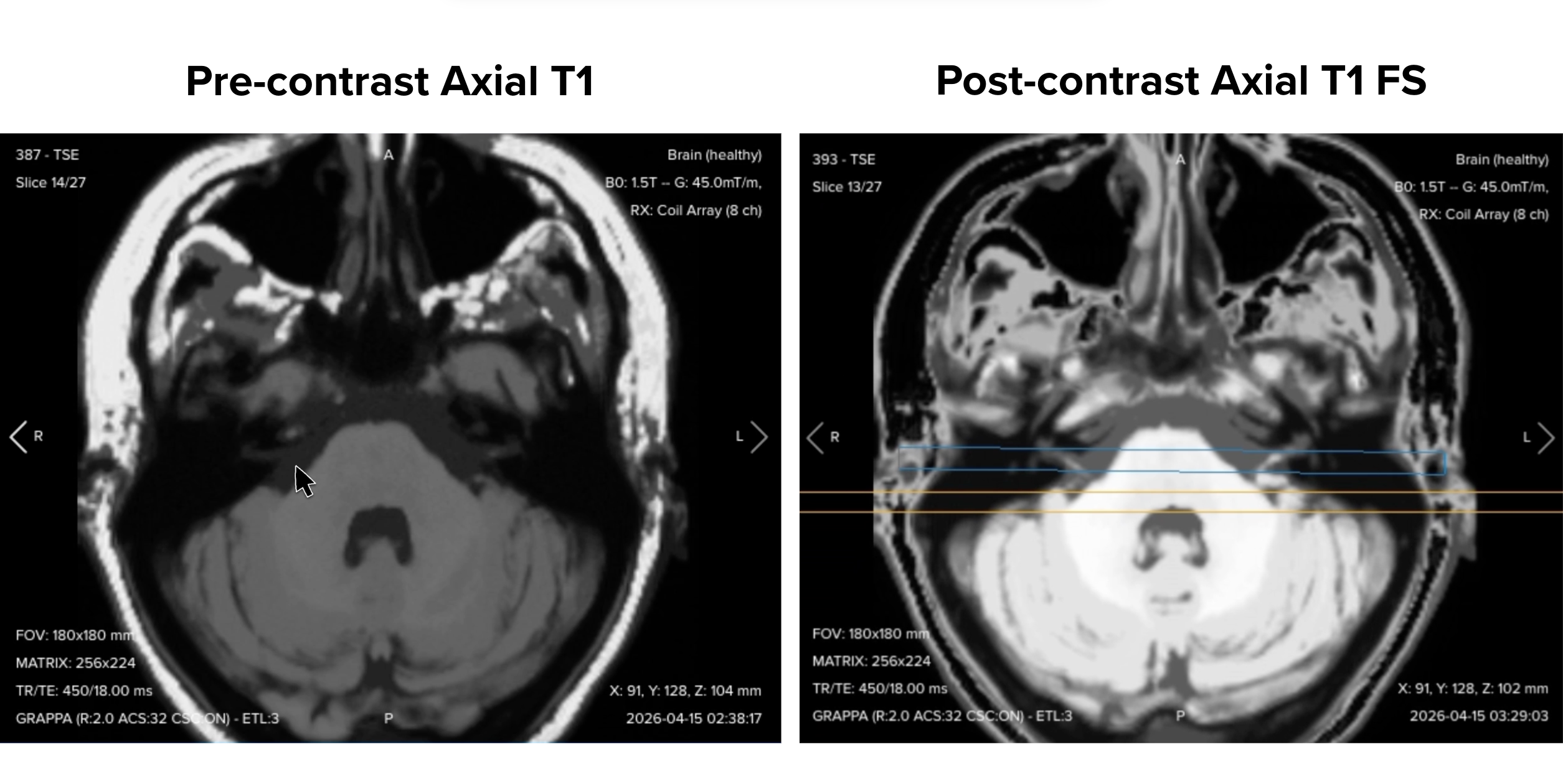
Comparison of pre-contrast axial T1 and post-contrast fat-suppressed axial T1 at the same slice position in an IAC MRI:
Line up the same slice number on the pre-contrast T1 and the post-contrast T1 FS. Subcutaneous fat should be bright on the native T1 and completely suppressed on the post-contrast image.
If the two stacks do not line up slice for slice, the radiologist cannot make a confident call on enhancement, and the study loses much of its value.
Final Checks
Before finishing an IAC/IAM MRI, always check these 5 points to ensure diagnostic quality:
Resolution: Cranial nerves VII and VIII must be sharply resolved against CSF on the 3D sequences. The bSSFP should deliver sub-millimeter isotropic voxels, and the 3D T2 TSE 1 mm isotropic voxels.
Coverage: All axial sequences must cover from the level of the hippocampus down to the foramen magnum or C1, and the coronals from the posterior sphenoid sinuses to the fourth ventricle.
Geometric Match: Post-contrast sequences must be an exact copy of the pre-contrast sequences, slice for slice.
Fat Suppression Quality: Post-contrast T1 FS images must show uniform suppression across the skull base, with no residual bright fat near the petrous apex.
Artifact Management: No motion blur, no banding across the canal, no wrap-around from the small field of view, and no susceptibility dropout at air and bone interfaces.

.svg)

.png)
.jpeg)

.png)
.png)