This step-by-step guide is for MRI students, radiographers, and technologists who wish to improve their planning skills and master the humerus MRI protocol.
What you will learn:
Key factors in humerus MRIs, including trade-offs.
Patient and scanner setup tips.
Best pulse sequences and planning techniques.
Ways to avoid common artifacts.
What great humerus images should look like.
Key Takeaways
Because we image a whole long bone across a 40 cm field of view, SNR generally comes first.
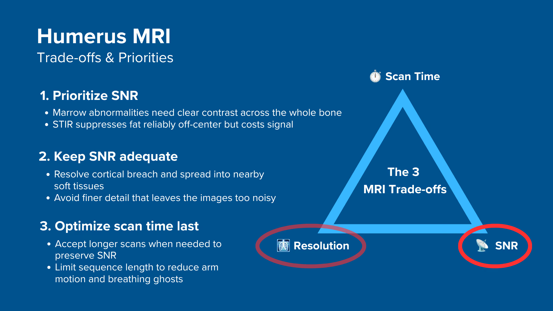
Marrow disease is found through contrast rather than fine detail, and STIR gives up signal to null fat reliably away from isocenter. We therefore typically 1) prioritize SNR, 2) keep resolution adequate for the clinical question, and 3) optimize scan time last. If the patient cannot hold the arm position, scan time moves up the list.
We use three contrasts across three planes.
T1 TSE maps the marrow and the anatomy along the full length of the bone. T2 TSE and STIR TSE are the fluid-sensitive sequences, with STIR suppressing the fat. Coronal and sagittal planes show length, the axial plane shows compartments.
Avoid these 5 common humerus artifacts.
In this protocol, geometry controls the artifacts more than the parameters do. The phase direction runs foot to head on the coronal and sagittal, anterior to posterior on the axials, and foldover suppression stays on in every plane.
Artifacts
Solution – How to Avoid It
Motion and respiratory ghosting
Support the arm, use anterior to posterior phase on the axials.
Flow and pulsation ghosting
Use foot to head phase on coronal and sagittal.
Wrap-around (aliasing)
Keep foldover suppression on in all planes.
Chemical shift misregistration
Keep bandwidth at 220 Hz/pixel or higher at 1.5 T.
Partial volume averaging
Add thin targeted slices for a focal finding.
STIR finds the lesion, T1 shows how far it extends.
STIR is the sequence that makes edema, infection and occult injury conspicuous once the bright fatty marrow is nulled. T1 is the sequence that tells the radiologist how far along the shaft an abnormality actually runs.
Intro to Humerus MRIs
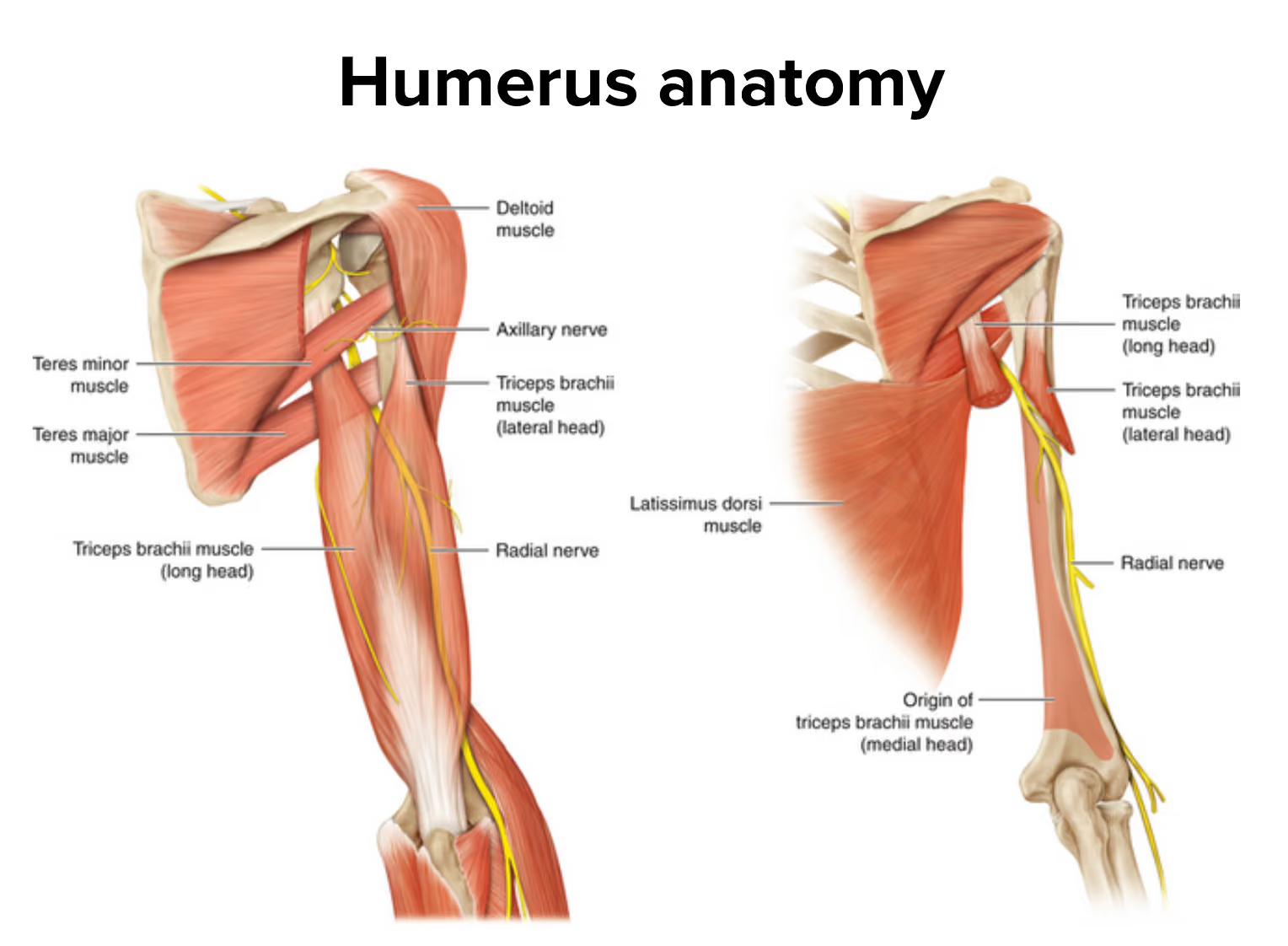
The humerus is the longest bone of the upper limb, running from the humeral head at the shoulder down to the elbow joint, roughly 30 cm in an adult. It is wrapped in the deltoid, biceps, and triceps, and it carries two structures that matter on every report: the radial nerve, which spirals around the posterior shaft in the spiral groove, and the brachial artery and vein, which run down the medial side of the arm.
What makes this study different from a shoulder or an elbow MRI is scale. We are not imaging a joint. We are imaging a whole long bone, which means every image has to stay diagnostic across a 40 cm field of view, while still showing the bone marrow, the cortex, and the surrounding soft tissues. Detail that looks excellent over one segment of the shaft is worthless if the rest of the bone is too noisy to read.
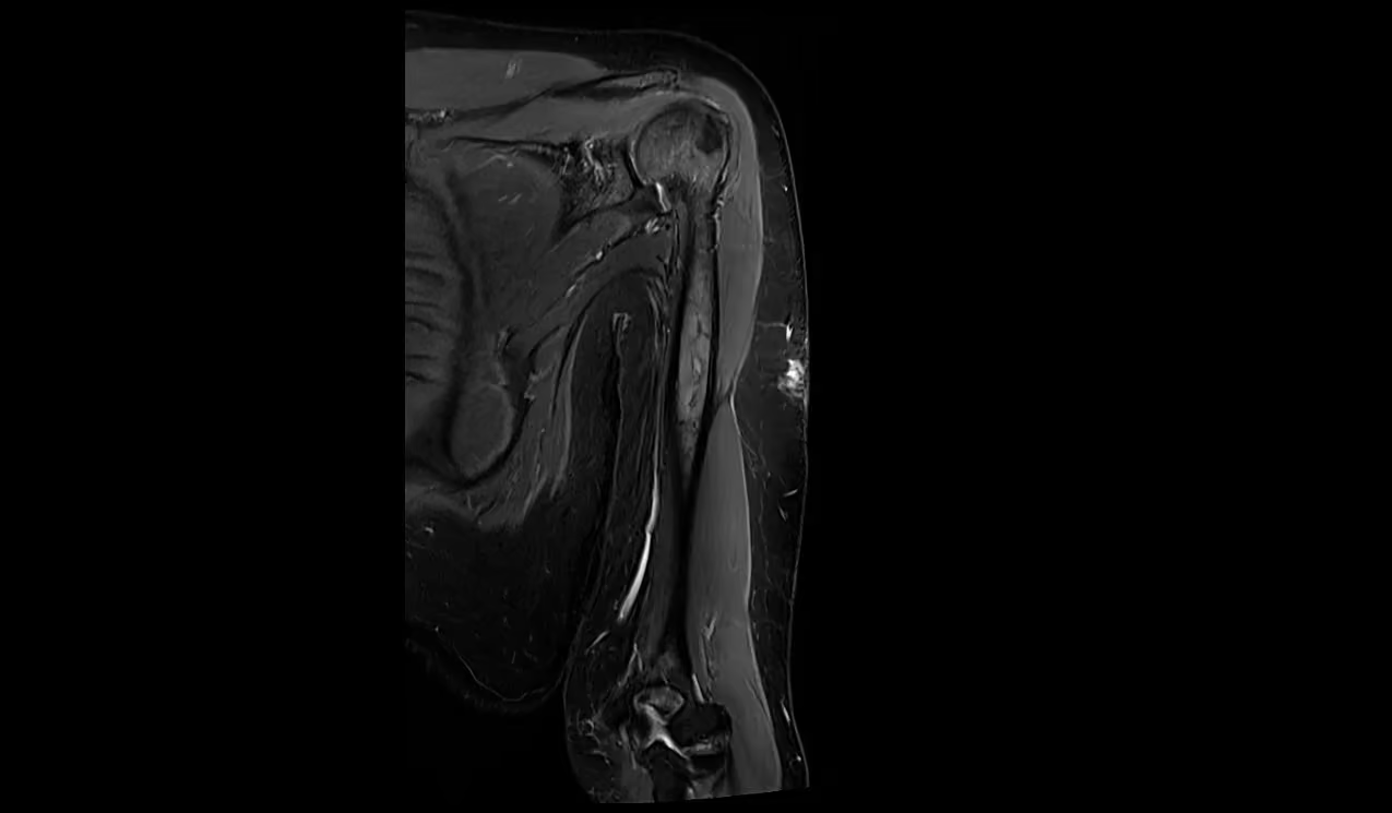
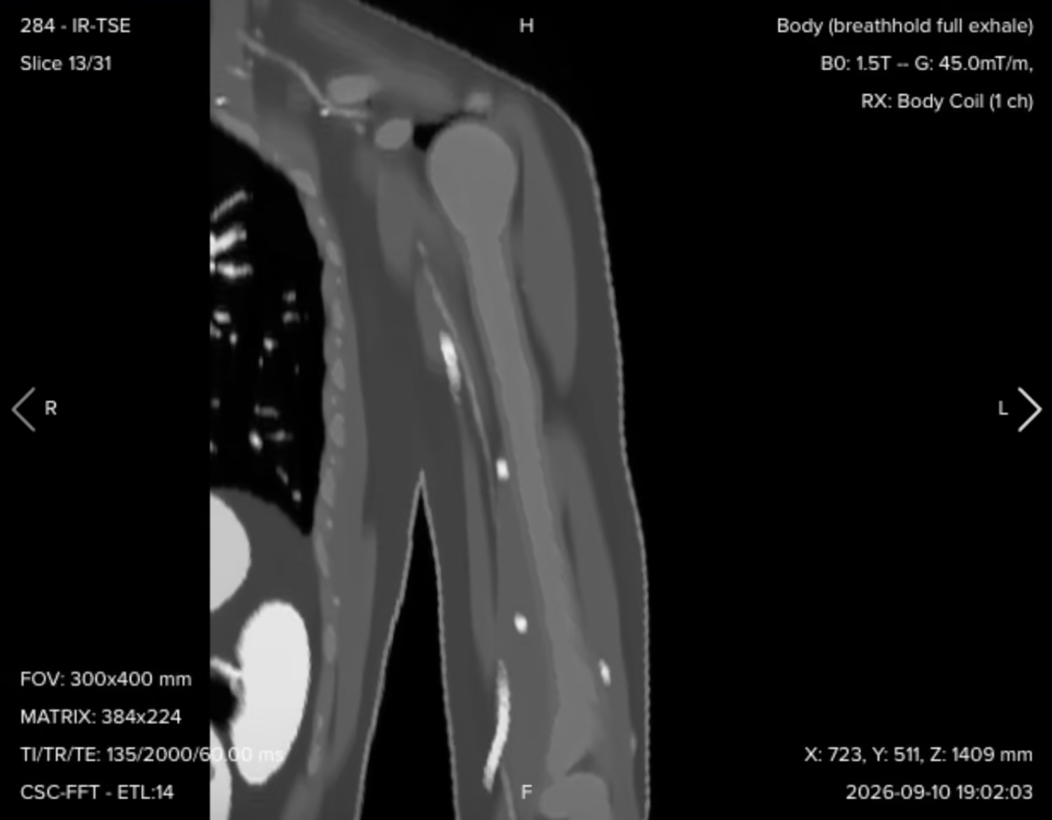
Coronal STIR of the full humerus from the humeral head to the elbow joint, showing the full 40 cm of coverage required in a single stack – Image credit: MRI Master
The study is usually requested for a suspected bone tumor, a metastasis or myeloma deposit, a pathological or occult fracture, osteomyelitis, or a soft tissue mass or muscle tear in the upper arm. A non-contrast protocol of three contrasts in three planes typically takes around 25 to 35 minutes of table time, depending on how many slices the axial coverage needs.
Why This Protocol Uses STIR Rather Than Spectral Fat Suppression
Both STIR and spectral fat saturation give you a fluid-sensitive image with the fat signal removed, but they do it in different ways, and in the upper arm that difference decides which one you can trust.
Spectral fat saturation works by targeting the fat resonance frequency directly. It needs a uniform main magnetic field over the anatomy to do that, because if the field drifts, the saturation pulse lands on the wrong frequency and suppression fails or becomes patchy.
The humerus sits off to the side of the bore, away from the magnet center, which is exactly where field uniformity is at its worst. STIR instead nulls fat by its T1 recovery using an inversion pulse, so it does not depend on the fat peak sitting at a predictable frequency. That makes it far more reliable in this position, and it is why STIR is the fluid-sensitive sequence in this protocol rather than a fat-saturated T2.
The cost is signal. The inversion pulse suppresses fat by nulling it, and that is signal you then have to win back through the rest of your parameter choices, which is the main reason SNR sits at the top of the trade-off list below.
How to Balance the 3 Trade-offs in Humerus MRIs
In MRI, we always face a trade-off between 3 key metrics:
Scan Time: How fast a pulse sequence can be completed.
Resolution: How much detail the image can display.
SNR: How clear the image is, meaning how much signal we have compared with noise.
Improving one of these metrics often reduces the performance of the others.
To decide what trade-offs to make, we must consider the needs of each clinical situation.
For humerus MRIs, we face these challenges:
We image a long bone from the shoulder to the elbow, so every image must stay diagnostic across a 40 cm field of view. Detail that is excellent over one segment of the shaft is worthless if the rest of the bone is too noisy to read.
The findings we look for are marrow replacement, edema, infection, and cortical breach, which we detect through tissue contrast rather than fine detail. We rely on STIR for the fluid-sensitive images, because the arm sits away from the magnet center where spectral fat suppression becomes unreliable. STIR nulls fat with an inversion pulse, and that pulse costs us signal we have to win back elsewhere.
The patient holds an awkward arm position for the whole study, and the chest sits centimeters from the anatomy. Long sequences invite both patient movement and respiratory ghosting.
Therefore, we typically:
Prioritize SNR to keep marrow and soft tissue contrast clear across the full length of the bone, and to compensate for the signal that STIR gives up.
Keep resolution adequate for the clinical question, which means enough in-plane detail to judge cortical involvement and the relationship of a lesion to nearby muscles, nerves, and vessels.
Optimize scan time last, while keeping each sequence short enough that the patient can hold the position without moving.
When a sequence runs long, reduce the matrix in the phase encoding direction rather than cutting signal averages. This shortens the scan and slightly increases SNR, at the cost of detail in one direction only. When a focal abnormality shows up on the survey images, go back and add thinner slices with a smaller field of view through that level.
Note! Prioritizing SNR in humerus MRIs is only a general guideline, NOT a strict rule. When the clinical question is a small cortical lesion or the exact margin of a soft tissue mass, resolution moves to the top and you accept a noisier image to get it. The right balance always depends on factors such as field strength, patient cooperation, available hardware, and the clinical question.
Humerus Health Conditions and the MRI Sequences That Reveal Them
The humerus MRI study can help us diagnose a wide range of health conditions. The table below lists some of the most common conditions and what pulse sequences reveal them.
In this protocol, T1 and T2 are both non-fat-suppressed and acquired without contrast. STIR provides the fat-suppressed fluid-sensitive images.
Common Humerus Conditions
Clearly Seen on Sequence
Why This Sequence?
Marrow replacement and structural lesions:
• Primary bone tumors
• Metastases and myeloma
• Pathological fractures
T1 TSE
Highlights fat and gives clear anatomical detail, so abnormal marrow stands out against normal marrow. Normal marrow in the adult humeral shaft is fatty and bright, so a tumor or a fracture line stands out dark against it. This makes T1 the best sequence for estimating how far a marrow abnormality runs along the bone.
Fluid-filled and cystic change:
• Bone cysts
• Cystic or necrotic tumor change
• Muscle tears
T2 TSE
Makes fluid bright against darker muscle and cortex, so cyst cavities, septations and fluid-fluid levels become visible. Because fat is not suppressed, the tissue planes around a lesion stay clear.
Edema, infection and occult injury:
• Occult and stress fractures
• Osteomyelitis
• Muscle injury and edema
STIR TSE
Suppresses fat with an inversion pulse, so bright fatty marrow no longer hides increased water content and subtle edema becomes obvious. Inversion recovery also works reliably when the arm sits off the magnet center, where spectral fat suppression tends to fail.
How to Perform a Humerus MRI
The step-by-step guide below will show you how to set up and perform a humerus MRI protocol in practice.
We will perform the protocol in 3 parts:
Set up the Patient and MRI Scanner
Plan and Acquire the Protocol Sequences
Review the Images
Part 1: Set up the Patient and MRI Scanner
1. Position the Patient in the Scanner
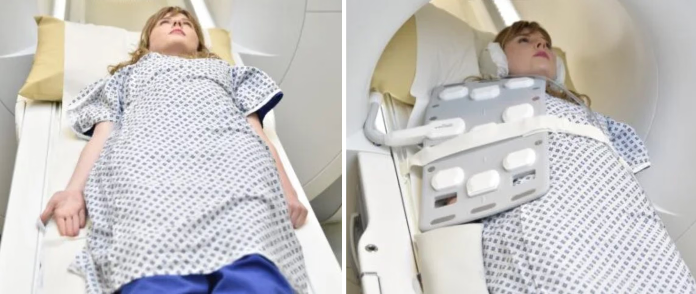
Lay the patient head-first and supine (on their back), with the arm of interest at the side in a neutral, thumb-up position, and center the laser over the mid humerus.
Motion control deserves real attention here. The patient has to hold an awkward arm position for the whole study, and if they are holding it in place by muscle effort, they will move. Pad and support the arm along its whole length so the position is passive, give a pillow under the head and a cushion under the knees, and tell the patient how long each sequence will run.
For long bone extremities in the upper limb, most facilities use the anterior coil combined with the spine coil, which gives good coverage and good signal across the whole region of interest. Some departments use a flexible coil instead, depending on the size of the patient's arm and the size of the coil. If you can wrap it around the entire anatomy of interest and still get rich signal, a flexible coil works well.
✅ Correct Patient Positioning:
Image credit: MRI Master
2. Check the Scanner's Hardware Settings
Once the patient is in place, review your scanner's hardware settings.
In this guide, we will use the following settings:
Scanner Setting
Value
Why This Value
Magnetic field strength
1.5 T
The most common clinical field strength for long bone imaging. The fat-water offset of about 220 Hz is easier to manage than at 3 T, and field uniformity holds up better with the arm positioned away from isocenter.
Maximum gradient strength
45 mT/m
Provides strong, versatile gradient performance that supports fast imaging and precise spatial encoding.
Coil
Body Rx
The simulator equivalent of the anterior plus spine coil combination most facilities use for upper limb long bones, giving good coverage and signal across the whole region of interest.
This hardware setup is widely used in clinical practice. It balances acquisition time, image quality, and patient comfort.
Remember that every parameter in this guide is tied to this hardware setup. Change the field strength, the gradient performance, or the coil and the optimal bandwidth, turbo factor, and acceleration factor all change with it.
3. Capture the Initial Localizer Images
Before we can perform any MRI protocol, we must always capture initial localizer images of the patient. These images act as a guide for planning the detailed scans we will perform next.
Select the region to cover the shoulder and the elbow together, set the isocenter over the mid-humerus, and run the standard three-plane survey.
We should always capture localizers in three planes:
Axial
Sagittal
Coronal
For a long bone, one survey set is often not enough. Depending on how the patient is lying, the survey may not show the complete long axis of the humerus in any single slice, and you cannot plan an angled coronal or sagittal from images that do not contain the bone you are angling to.
So before the high-resolution sequences, acquire a second, tailored set of localizers, one for each plane, angled to the patient's own humerus:
Coronal localizer: scroll the sagittal survey from the humeral head down to the elbow to find the direction the bone actually runs, then angle the coronal to that direction. Ten slices and a few seconds are enough.
Sagittal localizer: clone the coronal localizer, then use the coronal images you just acquired to angle the sagittal parallel to the humeral axis. Because it is a clone, this takes a couple of seconds to set up.
Axial localizer: clone again, and align the slices perpendicular to the humerus. Set a slice gap here. This is only a localizer, so a gap buys you wider coverage superiorly and inferiorly for the same handful of slices, which means nothing is missing when you plan the real sequences.
Rename each one as you go, so the three are easy to pick up later when you plan the high-resolution sequences.
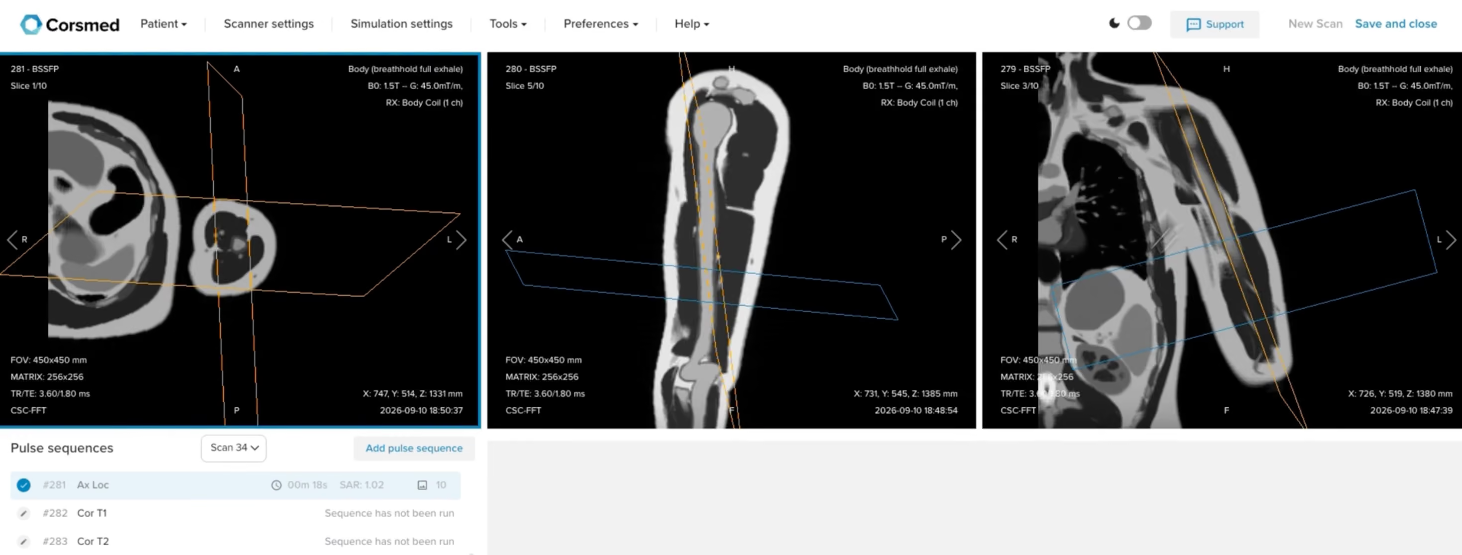
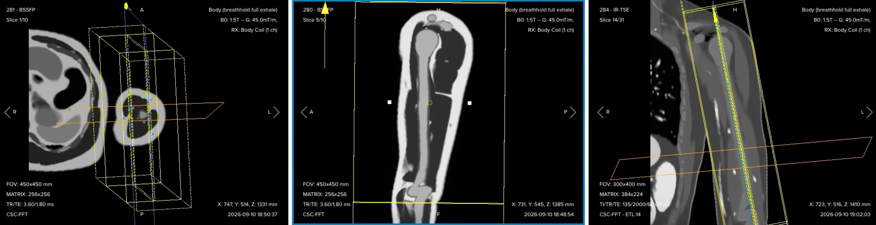
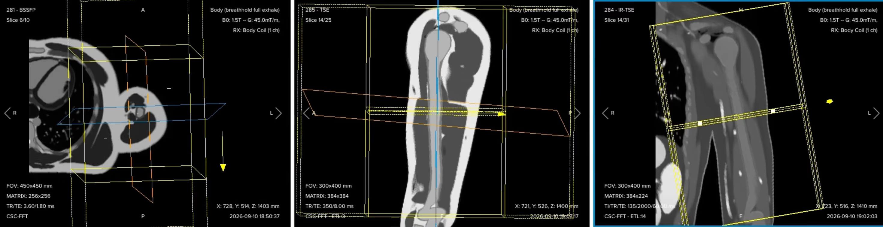
These are coarse, fast acquisitions, and they should stay that way. The coronal localizer in this guide uses a 450 × 450 mm field of view, a 256 × 256 matrix, 10 slices at 5 mm thickness with a 5 mm gap, which gives 1.76 × 1.76 × 5.00 mm voxels and an acquisition time of under 20 seconds. The equal gap and slice thickness is the point: it doubles the coverage for the same ten slices, which is exactly what you want from an image you are only going to plan from.
Before planning anything, check the sagittal localizer. It should show the entire humerus in one single slice. If it does, your coverage is good enough to plan every high-resolution sequence that follows.
✅ Correct setup of localizer images in the three viewports on the Corsmed MRI simulator:
Part 2: Plan and Acquire the Protocol Sequences
When all preparations are ready, we can start planning and acquiring the protocol sequences.
The 7 Sequences of a Standard Humerus MRI Protocol
Coronal T1 TSE
Coronal T2 TSE
Coronal STIR TSE
Sagittal T1 TSE
Sagittal STIR TSE
Axial STIR TSE
Axial T1 TSE
In musculoskeletal exams, we typically acquire three planes according to the structure of interest. Here, the coronal and sagittal planes show the length of the bone, and the axial plane shows the compartments in cross-section. Three contrasts cover the diagnostic ground: T1 for marrow and anatomy, T2 for fluid with the tissue planes preserved, and STIR for fluid with the fat nulled.
Keep in mind that this is a universal guideline, not a fixed standard. Your facility might run fewer or more sequences, or a different contrast in another plane. The way you angle and position them will be very similar either way.
A practical note on order. Once one plane is planned, you can copy that geometry to the other sequences in the same plane and run them while you plan the next plane. The protocol below follows that workflow: plan the coronals, set them running, then move to the sagittal and the axial.
The values in the tables below are worked examples for the 1.5 T setup used in this guide. Exact numbers vary by scanner, coil, and department, so treat them as a starting point rather than as fixed limits.
1. Coronal T1 TSE
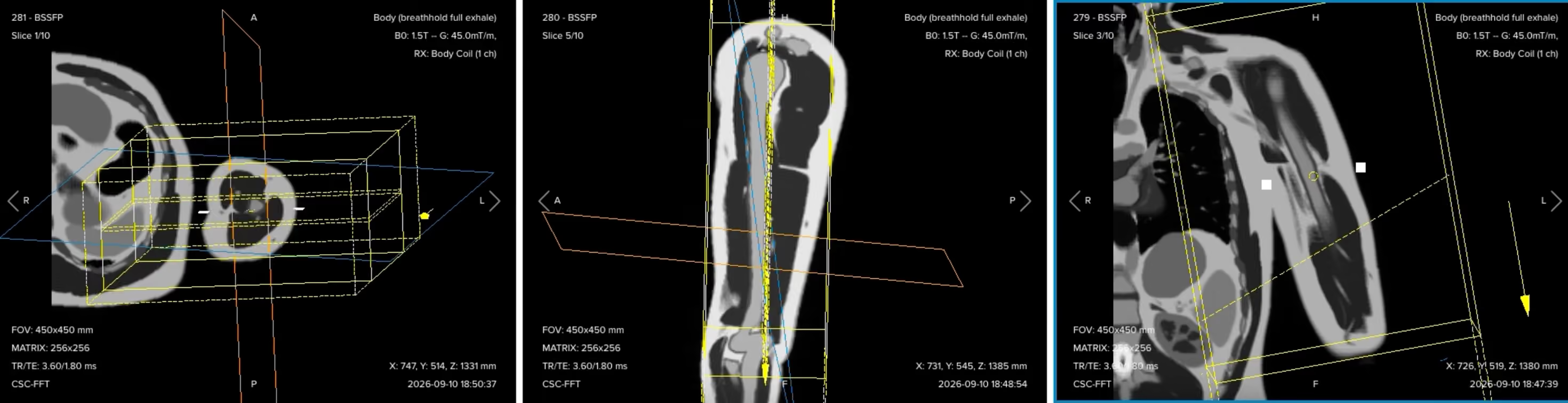
✅ Correct planning:
Planning Instructions:
Right-click on the coronal localizer and set the in-plane position, so you can see the field of view and position it over the bone.
Set a rectangular field of view. The humerus is long in one direction and short right to left, so we use 400 mm in the phase direction and 300 mm in the frequency direction.
Set the foldover direction to foot to head, so the larger 400 mm dimension runs along the length of the bone. These two settings are linked, and this is what covers the anatomy from superior to inferior.
Use the sagittal localizer for the angle. It shows the full extension of the humerus, so set the slice package completely parallel to the bone to unveil the whole shaft in one slice.
Use the axial localizer for the coverage. Add slices to cover the coronal plane from anterior to posterior, center the package, and verify that the slices run perpendicular to the scapular blade.
For presentation, align the displayed field of view along the humerus. The radiologist gets the correct anatomical angle and an image that is laid out the way they read it.
Parameters for Coronal T1 TSE:
Parameter
Recommended Values
Why These Values
Echo Time (TE)
8–12 ms
Short TE is required for T1 contrast.
Repetition Time (TR)
350–500 ms
Short TR is required for T1 contrast.
Field of View (FOV)
300 × 400 mm (frequency × phase)
Rectangular FOV matched to a long bone, with the 400 mm dimension along the shaft.
Matrix
384 × 384
Gives 0.78 × 1.04 mm in-plane voxels, enough to judge cortical margins across the full length.
Number of Slices
28–34
Covers the humerus from anterior to posterior with no gap in the stack.
Slice Thickness
4 mm
Thick enough to hold SNR across a 40 cm FOV, thin enough for marrow assessment.
Slice Gap
0.4 mm
10% of slice thickness, which limits cross-talk between adjacent slices.
NEX / Averages
1–2
A T1 image is already signal-rich, so one average keeps acquisition time reasonable.
Bandwidth per pixel
220–250 Hz/px
Set at or above the 220 Hz fat-water offset at 1.5 T, holding chemical shift to about one pixel.
Turbo Factor / ETL
3–5
Kept short so the effective TE stays short, preserving T1 weighting.
Parallel Imaging
None
SNR is the priority here, and acceleration would cost signal we need across the long FOV.
Foldover Direction (Phase)
Foot to head
Puts the 400 mm dimension along the bone and runs flow ghosts along the shaft.
Foldover Suppression
Yes
Anatomy continues above and below the FOV in the phase direction and would otherwise wrap.
Fat Suppression
None
Bright fatty marrow is the background that makes a dark lesion visible on T1.
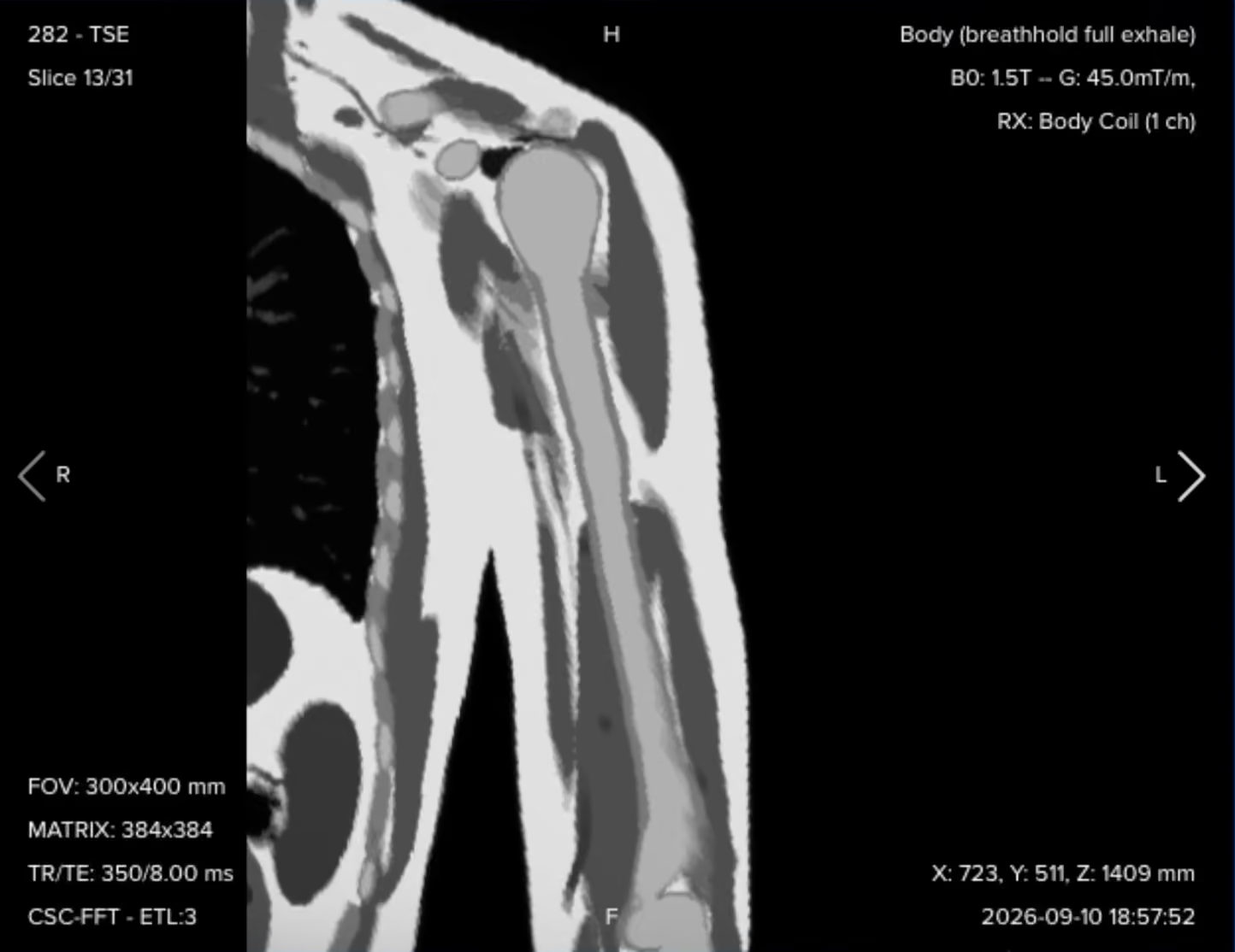
Resulting coronal T1 image:
Check that the whole shaft is in the image and that the marrow signal is uniformly bright. This series is your anatomical reference for everything that follows.
2. Coronal T2 TSE
✅ Correct planning:
Planning Instructions:
Do not re-plan this by hand. Right-click on the coronal T1, select Copy, then Custom, and continue.
Copying as Custom brings across all of the geometry, including the slice positions, so the T2 is an identical copy of the T1 planning.
Identical geometry is what lets the radiologist compare the two contrasts slice for slice.
Only the contrast parameters change, and those are already set for this sequence.
Parameters for Coronal T2 TSE:
Parameter
Recommended Values
Why These Values
Echo Time (TE)
90–110 ms
Long TE is required for T2 contrast.
Repetition Time (TR)
3,000–4,000 ms
Long TR is required for T2 contrast.
Field of View (FOV)
300 × 400 mm (frequency × phase)
Copied from the coronal T1 to keep geometry identical.
Matrix
384 × 384
Copied from the coronal T1.
Number of Slices
28–34
Copied from the coronal T1.
Slice Thickness
4 mm
Copied from the coronal T1.
Slice Gap
0.4 mm
Copied from the coronal T1.
NEX / Averages
1–2
One average is enough at this voxel size, and the long TR already carries the scan time.
Bandwidth per pixel
220–250 Hz/px
Chemical shift at the cortex-marrow boundary is held to about one pixel at 1.5 T.
Turbo Factor / ETL
20–25
A long echo train suits the long effective TE and keeps the scan near three minutes.
Parallel Imaging
None
Matches the coronal T1, and the sequence is already short enough without it.
Foldover Direction (Phase)
Foot to head
Copied from the coronal T1, keeping flow ghosts along the bone.
Foldover Suppression
Yes
Shoulder and forearm anatomy continues past the FOV edges in the phase direction.
Fat Suppression
None
Leaving fat bright keeps the tissue planes around a lesion visible.
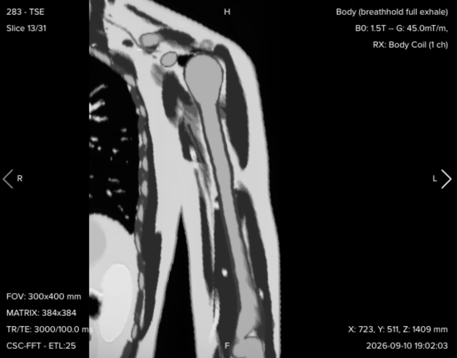
Resulting coronal T2 image:
The geometry is copied, the contrast parameters are already optimized, and the resolution is preserved along with it. Signal, voxel size and acquisition time all land in a reproducible place.
3. Coronal STIR TSE
✅ Correct planning:
Planning Instructions:
Copy the geometry again, from either the coronal T1 or the coronal T2, since their planning is identical.
What changes here is the contrast. STIR is a hybrid weighting, with an effective TE that sits between proton density and T2, and a repetition time to match.
Set the inversion time for your field strength. At 1.5 T, use 130 to 150 ms depending on your radiologist's preference. We use 135 ms here.
STIR runs longer than T1 and T2 because of the inversion pulse. If you need to bring the time down, reduce the matrix in the phase direction rather than cutting averages, then check that the voxel size still answers the clinical question. Reducing the phase matrix from 384 to 224 keeps this sequence at four minutes.
Parameters for Coronal STIR TSE:
Parameter
Recommended Values
Why These Values
Echo Time (TE)
50–70 ms
An intermediate TE gives the hybrid proton density to T2 weighting STIR is read with.
Repetition Time (TR)
2,000–3,000 ms
Long enough for full longitudinal recovery between inversion pulses.
Inversion Time (TI)
130–150 ms
Nulls fat at 1.5 T, where fat recovers through zero at around this time.
Field of View (FOV)
300 × 400 mm (frequency × phase)
Copied from the coronal T1 so the three contrasts line up.
Matrix
384 × 224
Phase matrix reduced to hold the scan at four minutes, giving 0.78 × 1.79 mm voxels.
Number of Slices
28–34
Copied from the coronal T1, covering anterior to posterior.
Slice Thickness
4 mm
Copied from the coronal T1.
Slice Gap
0.4 mm
Copied from the coronal T1.
NEX / Averages
1–2
The larger phase voxel already recovers signal, so one average holds the time down.
Bandwidth per pixel
200–220 Hz/px
Fat is nulled here, so chemical shift is not a concern and the lower bandwidth buys back SNR.
Turbo Factor / ETL
12–16
Matched to the intermediate effective TE, and keeps the inversion-recovery scan practical.
Parallel Imaging
None
STIR has already given up signal to the inversion pulse, so we do not spend more.
Foldover Direction (Phase)
Foot to head
Copied from the coronal T1, running brachial vessel ghosts along the shaft.
Foldover Suppression
Yes
Anatomy extends past the FOV above and below in the phase direction.
Fat Suppression
Inversion recovery (STIR), TI 135 ms
Nulls fat by T1 recovery, which stays reliable with the arm away from isocenter.
Resulting coronal STIR image:
Check the fat suppression first. Marrow and subcutaneous fat should both be dark and evenly suppressed along the whole bone. With the coronals planned, set them running while you move on to the sagittal and axial planes.
4. Sagittal T1 TSE
✅ Correct planning:
Planning Instructions:
The geometry follows the same logic as the coronal. The sagittal is long foot to head and short anterior to posterior, so we keep the rectangular field of view and set the foldover direction foot to head again, putting 400 mm along the bone and 300 mm across it.
Right-click on the sagittal localizer and set the in-plane position, then check that the rectangle covers the humeral head at the top and reaches the elbow joint at the bottom.
Use your high-resolution coronal images for the angle, not the localizer. Scroll to the middle slice where the shaft is best seen, then use the handles to set the slice package parallel to the bone.
From the same coronal, add enough slices to cover the bone right to left, checking that nothing is cut off on either side.
Confirm on the axial that the slices run parallel to the plane of the bone there too.
Parameters for Sagittal T1 TSE:
Parameter
Recommended Values
Why These Values
Echo Time (TE)
8–12 ms
Short TE is required for T1 contrast.
Repetition Time (TR)
350–500 ms
Short TR is required for T1 contrast.
Field of View (FOV)
300 × 400 mm (frequency × phase)
Rectangular again, with the long dimension foot to head along the bone.
Matrix
384 × 384
Gives 0.78 × 1.04 mm voxels, matching the coronal so image quality is equal across planes.
Number of Slices
22–28
Covers the humerus right to left, which needs fewer slices than the coronal direction.
Slice Thickness
4 mm
Matched to the coronal so the two planes are read at the same resolution.
Slice Gap
0.4 mm
10% of slice thickness, which limits cross-talk between adjacent slices.
NEX / Averages
1–2
One average is enough on a signal-rich T1 and keeps the sequence under three minutes.
Bandwidth per pixel
220–250 Hz/px
At or above the 220 Hz fat-water offset at 1.5 T, limiting chemical shift to about one pixel.
Turbo Factor / ETL
3–5
Short echo train protects the short effective TE that gives T1 weighting.
Parallel Imaging
None
Consistent with the coronal T1, keeping full signal across the long FOV.
Foldover Direction (Phase)
Foot to head
Aligns the phase direction with brachial blood flow, so flow ghosts run along the bone.
Foldover Suppression
Yes
Anatomy continues below the FOV toward the forearm and would otherwise fold in.
Fat Suppression
None
Bright marrow fat is what a dark lesion is read against on T1.
Resulting sagittal T1 image:
This is a good point to look at two linked settings. The foldover direction is foot to head, and that is the direction that carries both wrap and ghosts. Anatomy is not fully covered inferiorly, so wrap is a real risk, which is why foldover suppression is set to yes and the reading area is extended. At the same time, blood in this arm flows along the superior-to-inferior axis, so putting the phase direction along the flow keeps pulsation ghosts running up and down the bone rather than across it. One setting handles two artifacts.
5. Sagittal STIR TSE
✅ Correct planning:
Planning Instructions:
Once the sagittal T1 has reconstructed, right-click on it, select Copy, then Custom, and carry over the geometry and center position.
Keep the contrast identical to the coronal STIR: the same inversion time of 135 ms, the same effective TE and the same TR. Consistency between planes is what lets the radiologist read the same contrast the same way in every view.
Check the turbo factor under the Special tab, which should match the effective TE as it does on the coronal STIR.
As on the coronal STIR, reduce the phase matrix before saving to bring the acquisition time down while keeping the voxel size within what the radiologist needs.
Parameters for Sagittal STIR TSE:
Parameter
Recommended Values
Why These Values
Echo Time (TE)
50–70 ms
Identical to the coronal STIR, so the contrast reads the same in both planes.
Repetition Time (TR)
2,000–3,000 ms
Allows full longitudinal recovery between successive inversion pulses.
Inversion Time (TI)
130–150 ms
The same 135 ms null point used on the coronal STIR at 1.5 T.
Field of View (FOV)
300 × 400 mm (frequency × phase)
Copied from the sagittal T1 to keep the two sagittal contrasts aligned.
Matrix
384 × 224
Phase matrix reduced for acquisition time, giving 0.78 × 1.79 mm in-plane voxels.
Number of Slices
22–28
Copied from the sagittal T1, covering the bone right to left.
Slice Thickness
4 mm
Copied from the sagittal T1.
Slice Gap
0.4 mm
Copied from the sagittal T1.
NEX / Averages
1–2
One average, with the wider phase voxel supplying the signal instead.
Bandwidth per pixel
200–220 Hz/px
With fat nulled there is no fat-water boundary to misregister, so SNR wins here.
Turbo Factor / ETL
12–16
Aligned to the intermediate effective TE, matching the coronal STIR.
Parallel Imaging
None
No acceleration on a sequence that has already spent signal on the inversion pulse.
Foldover Direction (Phase)
Foot to head
Copied from the sagittal T1, keeping flow ghosts along the axis of the vessels.
Foldover Suppression
Yes
Uncovered anatomy above and below the FOV would otherwise alias into the image.
Fat Suppression
Inversion recovery (STIR), TI 135 ms
Same null point as the other two STIRs, so edema looks the same in every plane.
Resulting sagittal STIR image:
Compare this against the coronal STIR. The suppression quality and the brightness of any abnormal signal should look the same in both planes, because the inversion time and the contrast parameters are the same.
6. Axial STIR TSE
✅ Correct planning:
Planning Instructions:
The axial uses a square field of view of 240 × 240 mm. A rectangle gains you nothing here, because the arm in cross-section is close to square.
Set the foldover direction anterior to posterior, not right to left. The chest sits right next to the arm, so if the phase direction ran right to left, respiratory ghosts would travel straight across the humerus. Running them front to back moves them off the anatomy, which sits laterally.
Keep foldover suppression on. Turn it off in the simulator and you can watch the extended reading area disappear, leaving anterior and posterior tissue free to wrap into the middle of the image.
Right-click on the axial localizer to set the in-plane position, then use the coronal and sagittal high-resolution images to set the slice package exactly perpendicular to the long axis of the humerus. Confirm the perpendicular angle in both planes.
Add enough slices to cover from the acromioclavicular joint down to the elbow joint, which is the exploratory coverage the whole region needs. Switch to Tools, Display Options, View Mode, Slice View if you want to see the individual slices rather than the box, and check where each one bisects the anatomy.
Remember what this coverage is for. It is an exploratory axial of the whole region. If a mass or another focal abnormality turns up, that calls for thin slices through the structure and the tissue around it, planned for that individual patient.slice thickness and slice gap to manage the time this coverage costs. A 7 mm slice with a 2 mm gap is a survey setting, and it is a deliberate choice: it covers the whole bone without adding scan time through extra slices.
Parameters for Axial STIR TSE:
Parameter
Recommended Values
Why These Values
Echo Time (TE)
50–70 ms
The same intermediate TE as the coronal and sagittal STIR, for one consistent contrast.
Repetition Time (TR)
2,000–3,000 ms
Long enough for longitudinal recovery before the next inversion pulse.
Inversion Time (TI)
130–150 ms
The same 135 ms fat null used in the other two planes at 1.5 T.
Field of View (FOV)
240 × 240 mm
Square FOV matched to the roughly square cross-section of the upper arm.
Matrix
320 × 256
Gives 0.75 × 0.94 mm voxels, the highest in-plane detail in the protocol.
Number of Slices
38–44
Needed to reach from the acromioclavicular joint all the way down to the elbow.
Slice Thickness
7 mm
A survey thickness that covers the whole bone and holds SNR at this small voxel area.
Slice Gap
2 mm
Extends coverage over the full arm length without paying for additional slices.
NEX / Averages
1–2
One average, since the slice count already makes this the longest sequence.
Bandwidth per pixel
200–220 Hz/px
Fat is nulled, so bandwidth can stay low and return signal to a thin-voxel acquisition.
Turbo Factor / ETL
14–18
Long enough to make the slice count practical, short enough to hold the STIR contrast.
Parallel Imaging
None
The inversion pulse and the small voxels already cost signal we cannot afford to lose.
Foldover Direction (Phase)
Anterior to posterior
Sends respiratory ghosts from the chest front to back, away from the laterally placed arm.
Foldover Suppression
Yes
Anterior and posterior tissue sits outside the 240 mm FOV and would wrap into it.
Fat Suppression
Inversion recovery (STIR), TI 135 ms
Makes edema and fluid conspicuous in cross-section, reliably away from isocenter.
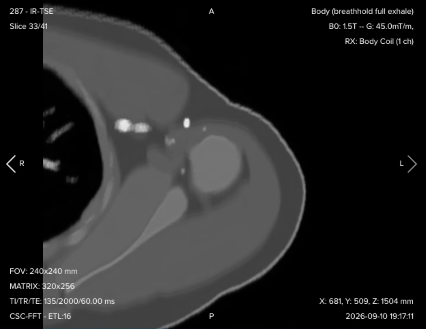
Resulting axial STIR image:
This sequence runs longer than the others, because of the inversion pulse, the signal it has to recover, and a slice count well above the coronal and sagittal. That is expected. The job is to keep the whole protocol balanced enough to stay reproducible.
7. Axial T1 TSE
✅ Correct planning:
Planning Instructions:
Copy the geometry and position from the axial STIR, so the two axial series line up slice for slice.
Only the contrast changes. A short TE and short TR give the T1 weighting, and the turbo factor follows that short effective TE.
Check that the bandwidth per pixel stays at or above 220 Hz/px. Fat is bright again on this sequence, so chemical shift at the fat-marrow and fat-muscle boundaries is back in play.
Leave foldover suppression on, for the same reason as on the axial STIR.
Parameters for Axial T1 TSE:
Parameter
Recommended Values
Why These Values
Echo Time (TE)
8–12 ms
Short TE is required for T1 contrast.
Repetition Time (TR)
350–500 ms
Short TR is required for T1 contrast.
Field of View (FOV)
240 × 240 mm
Copied from the axial STIR so the two cross-sectional series match.
Matrix
320 × 256
Copied from the axial STIR, giving 0.75 × 0.94 mm voxels.
Number of Slices
38–44
Copied from the axial STIR, covering acromioclavicular joint to elbow.
Slice Thickness
7 mm
Copied from the axial STIR.
Slice Gap
2 mm
Copied from the axial STIR.
NEX / Averages
1–2
One average is enough on a signal-rich T1 across this many slices.
Bandwidth per pixel
220–250 Hz/px
Fat is bright again here, so bandwidth returns to the 220 Hz offset at 1.5 T.
Turbo Factor / ETL
3–5
Short echo train keeps the effective TE short and the T1 weighting clean.
Parallel Imaging
None
Consistent with the rest of the protocol, where SNR is the priority.
Foldover Direction (Phase)
Anterior to posterior
Copied from the axial STIR, keeping chest ghosts off the arm.
Foldover Suppression
Yes
Chest and posterior tissue outside the square FOV would otherwise alias in.
Fat Suppression
None
Bright fat is what separates muscle groups and outlines the neurovascular bundle.
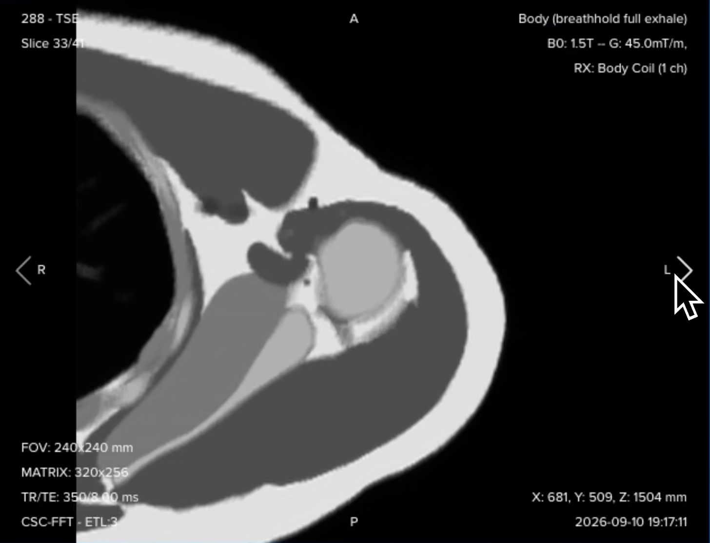
Resulting axial T1 image:
With the geometry copied from the STIR, these two axial series can be scrolled side by side at the same slice position, which is exactly how the radiologist will compare them.
How to Avoid Artifacts When Planning the Sequences
The table below lists the 5 common humerus artifacts, and what techniques you can use to avoid them:
Artifacts
Solution – How to Avoid It
Motion and respiratory ghosting
The patient holds an awkward arm position for the whole study, and the chest sits centimeters from the anatomy, so both movement and breathing throw ghosts along the phase direction. Pad and support the arm so the position is passive, set the phase direction anterior to posterior on the axials, and add a saturation band over the chest if ghosting persists.
Flow and pulsation ghosting
The brachial vessels run the length of the arm, and their pulsation repeats along the phase direction, which can lay ghosts straight across the bone. Set the phase direction foot to head on the coronal and sagittal so the ghosts run along the shaft instead, then check where they land and add flow compensation if they still cover the anatomy.
Wrap-around (aliasing)
The 40 cm coronal and sagittal field of view still leaves anatomy uncovered above and below, and the chest can fold into the 24 cm axial field of view. Keep foldover suppression enabled in all three planes, since enlarging the field of view instead fixes the wrap but coarsens resolution at the same matrix.
Chemical shift misregistration
Bright and dark bands appear where fat meets water, such as cortex against marrow, because the two resonate about 220 Hz apart at 1.5 T. Keep bandwidth at 220 Hz per pixel or higher on T1 and T2 to hold the shift to about one pixel, and go higher only when needed, since bandwidth costs SNR.
Partial volume averaging
Thick axial slices with a gap cover the whole bone efficiently, but a small lesion can blend into surrounding tissue or fall between slices. Never call a small finding from the survey axials alone, and instead add thinner slices with a smaller field of view through the level of concern, since widening the gap only reduces cross-talk.
Metal implants change the priorities. Plates, nails and prostheses cause signal voids, pileup and distortion. Use turbo spin echo rather than gradient echo, raise the receive bandwidth, and use thinner slices. On coronal and sagittal images, align the frequency encoding direction with the long axis of the implant. Keep fat suppression on STIR, and use SEMAC or MAVRIC when standard adjustments are not enough.
Part 3: Review the Images
Finally, we will review the images to ensure all the anatomical information we need is clear.
These key structures must be clearly visible in a humerus MRI:
The full humerus from the humeral head to the elbow joint, in one continuous stack
Bone marrow signal along the entire shaft
The cortical margins, anterior, posterior, medial and lateral
The individual muscle compartments of the upper arm
The neurovascular bundle and its relationship to the bone
Subcutaneous fat and the overlying soft tissues
The shoulder and elbow joints at the two ends of the coverage
Below, we will go through all the different image contrasts and explain their specific role in imaging the humerus.
T1 TSE – Marrow, Cortex, and the Extent of a Lesion
T1-weighted imaging makes fat appear bright and fluid dark. This contrast is ideal for fat-rich tissues and structural abnormalities.
In humerus MRI, T1 is where the radiologist judges extent. Normal adult shaft marrow is fatty and bright, so anything that replaces it reads as a dark segment against a bright background, and the length of that dark segment is the length of the disease.
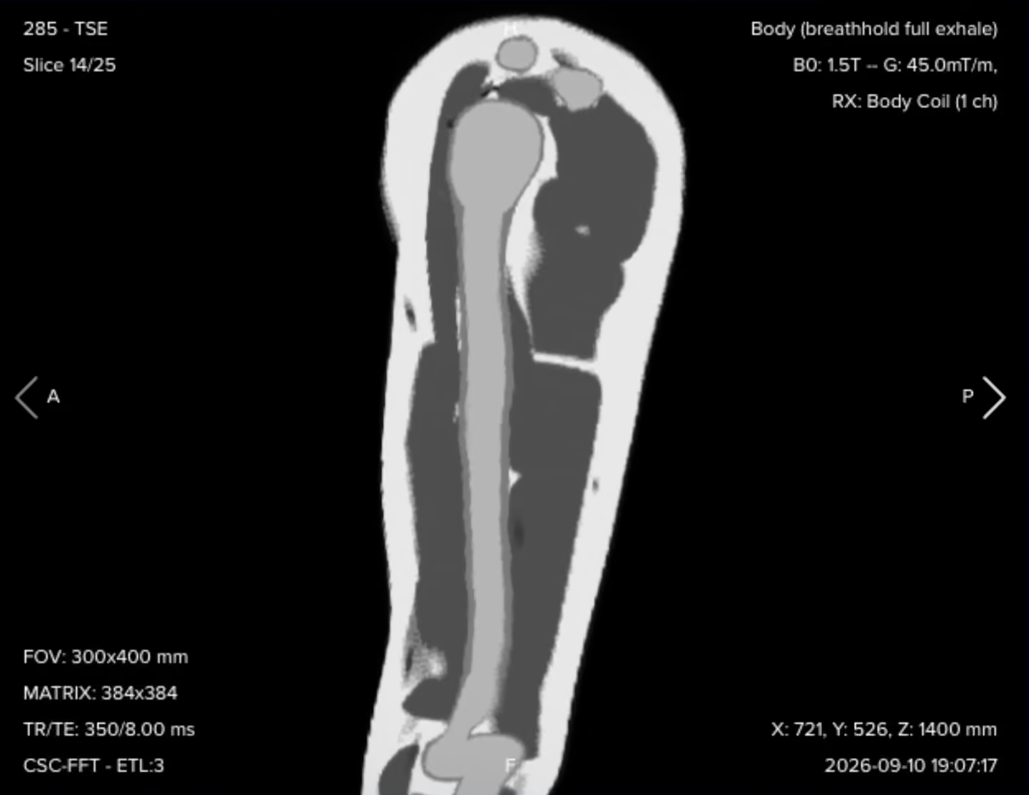
✅ Coronal T1 TSE – Correct Image Example:
Things to look for in Coronal T1:
An anatomical overview of the entire humerus and the surrounding soft tissues in one plane.
Normal fatty marrow signal, read against any area of marrow replacement.
Clearly defined cortical margins along the whole shaft.
The longitudinal extent of any marrow abnormality, which is the main question this sequence answers.
✅ Sagittal T1 TSE – Correct Image Example:
Things to look for in Sagittal T1:
A second anatomical plane for the marrow, the cortex and the muscles.
The anterior to posterior location of a lesion, which a coronal plane alone cannot fully characterize.
Longitudinal relationships that confirm what the coronal showed.
✅ Axial T1 TSE – Correct Image Example:
Things to look for in Axial T1:
Detailed cross-sectional anatomy, with fatty marrow, cortex, muscle groups and subcutaneous fat clearly separated.
The precise anatomical compartment a lesion sits in.
The neurovascular structures and how close they run to any abnormality.
A clean anatomical reference to compare against the axial STIR at the same slice.
T2 TSE – Fluid With the Tissue Planes Preserved
T2-weighted imaging makes fluids appear bright. This contrast is ideal for tissues and abnormalities with high water content.
In humerus MRI, the coronal T2 gives fluid-sensitive contrast across a large longitudinal portion of the arm. Because it is not fat-suppressed, it keeps the contrast between fat, muscle, marrow and fluid, so the tissue planes around a lesion stay readable while the fluid itself is bright.
✅ Coronal T2 TSE – Correct Image Example:
Things to look for in Coronal T2:
Fluid-containing abnormalities and areas of increased tissue water, bright against darker muscle and cortex.
Internal detail inside a cystic lesion, such as septations and fluid-fluid levels.
Preserved fat signal, which keeps the planes between muscle, marrow and lesion visible.
Findings that complement the tissue characterization from the T1.
STIR TSE – Edema, Infection, and Occult Injury
STIR removes the fat signal with an inversion pulse, so water-rich tissue stands out against a nulled background. This contrast is the most sensitive in the protocol to increased water content.
In humerus MRI, STIR is the detection sequence. Bright fatty marrow is what normally hides subtle edema, and once it is suppressed, bone marrow edema, inflammation, infection, occult stress injury, soft tissue edema and neoplastic change all become conspicuous along the full length of the bone.
✅ Coronal STIR TSE – Correct Image Example:
Things to look for in Coronal STIR:
Uniform fat suppression in both the marrow and the subcutaneous fat, along the whole bone.
Any bright marrow signal, which on this sequence means increased water content.
Broad longitudinal coverage, so nothing between the shoulder and the elbow is missed.
Soft tissue edema around the bone as well as inside it.
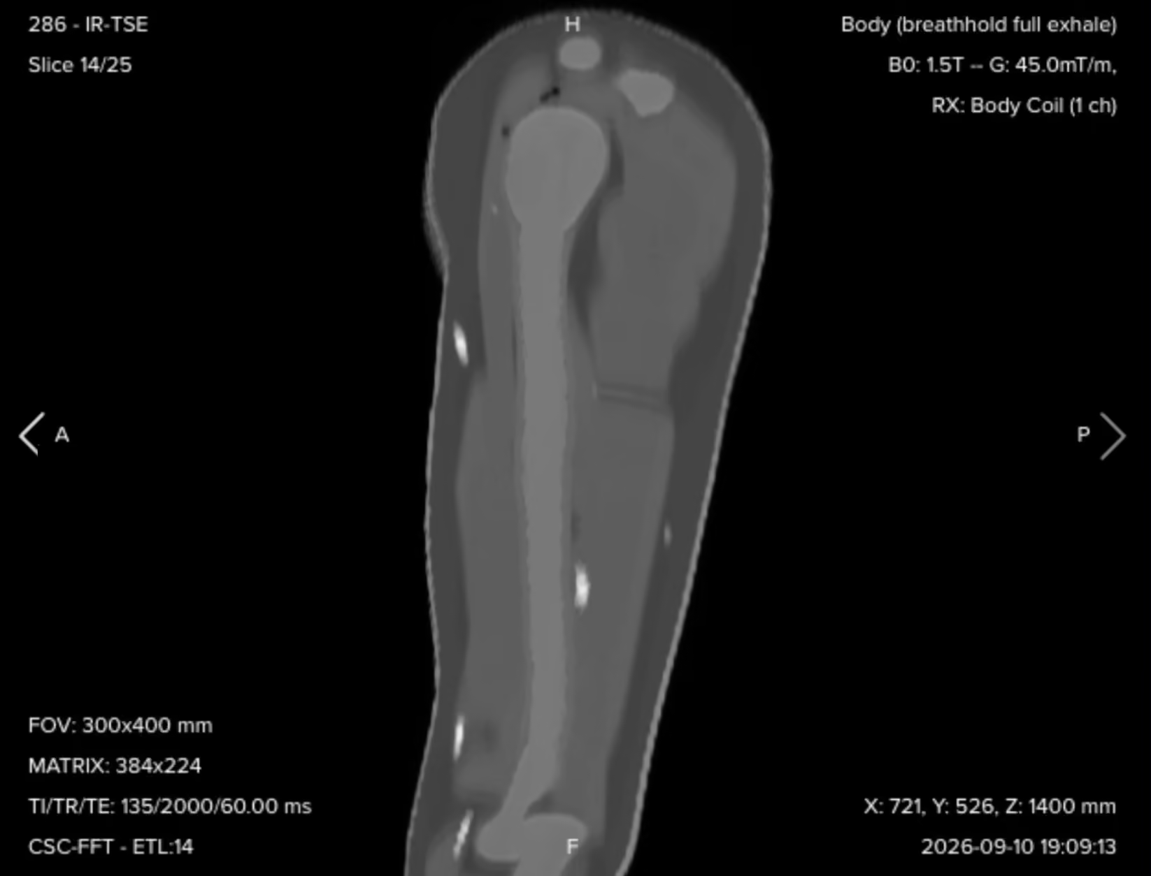
✅ Sagittal STIR TSE – Correct Image Example:
Things to look for in Sagittal STIR:
The anterior to posterior extent of marrow or soft tissue abnormality.
The full margins of edema, inflammation or a soft tissue lesion, read together with the coronal.
Suppression quality matching the coronal STIR, since the inversion time is the same.
✅ Axial STIR TSE – Correct Image Example:
Things to look for in Axial STIR:
The cross-sectional extent of pathology, which is what this plane is for.
Which individual muscle compartments are involved.
Involvement of the surrounding soft tissues and the neurovascular regions.
The relationship between a lesion and the humerus itself.
Full coverage when you scroll superiorly, all the way to the acromioclavicular joint.
Final Checks
Before finishing a humerus MRI, always check these 5 points to ensure diagnostic quality:
Coverage: The coronal and sagittal stacks must show the humerus from the humeral head to the elbow joint, and the axial stack must reach from the acromioclavicular joint down to the elbow.
Angulation: Coronal and sagittal slices parallel to the long axis of the humerus, axial slices perpendicular to it, each confirmed in a second plane before you save.
Fat Suppression: All three STIR series must show even suppression of marrow and subcutaneous fat along the whole bone, using the same inversion time in every plane.
Signal Across the Full Length: The marrow and soft tissue contrast must stay readable from the shoulder to the elbow, not only in the mid shaft where the coil sits best.
Artifact Management: No motion or respiratory ghosting over the arm, no wrap from outside the field of view in any plane, and no chemical shift banding at the cortex-marrow boundary on T1 and T2.