How to Plan a Brain Tumor MRI Protocol (Part 1: Pre-Contrast)

This step-by-step guide is for MRI students, radiographers, and technologists who wish to improve their planning skills and master the brain tumor MRI protocol.

What you will learn:

1. Key factors in brain tumor MRIs, including trade-offs.
2. Patient and scanner setup tips.
3. Best pulse sequences and planning techniques.
4. Ways to avoid common artifacts.
5. Qualities of great brain tumor images.

The brain is the control center for all body functions, processing sensory information and enabling cognitive abilities. Brain tumors, whether primary or metastatic, can severely disrupt these functions and present life-threatening complications.

Brain tumor MRI protocols are one of the most comprehensive imaging studies in MRI, often taking 30–45 minutes to complete. These protocols are designed to characterize lesions, assess their extent, plan treatment, and monitor response to therapy.

Accurate tumor diagnosis requires multiple sequences that provide complementary information about tumor composition, vascularity, and relationship to surrounding structures.

How to Balance the 3 Trade-offs in Brain Tumor MRIs

In MRI, we always face a trade-off between 3 key metrics:

• Scan Time: How fast a pulse sequence can be completed.
• Resolution: How much detail the image can display.
• SNR: How clear the image is, how much signal relative to noise.

Improving one of these metrics reduces the performance of the others. To decide what trade-offs to make, we must consider the needs of each clinical situation.

For brain tumor MRIs, we face these challenges:

• Missing a 2 mm metastasis could change treatment entirely. We need to see small lesions clearly and detect infiltrative margins that extend into normal brain tissue.
• We must differentiate between different tumor types based on their signal characteristics. This requires adequate image clarity to distinguish subtle differences in tissue properties.
• Brain tumor protocols are comprehensive studies that include many sequences. Most patients can tolerate around 30 minutes of scanning, but beyond that, motion artifacts can make images completely unreadable.

Therefore, we typically:

1. Prioritize resolution to detect small metastases and infiltrative margins,
2. Keep good SNR to ensure adequate image clarity for our resolution targets, and
3. Optimize scan time as needed to stay within the practical limit of around 30 minutes.

Brain Tumor Conditions and the MRI Sequences That Reveal Them

The brain tumor MRI study can help us diagnose a wide range of conditions. The table below lists the most common conditions and what pulse sequences reveal them:

How to Perform a Brain Tumor MRI

The step-by-step guide below will show you how to set up and perform a brain tumor MRI protocol in practice.

This tutorial is Part 1, covering pre-contrast sequences only. Part 2 will cover contrast injection, post-contrast sequences, and complete image review.

We will perform the protocol in 3 parts:

1. Set up the Patient and MRI Scanner
2. Plan and Acquire the Protocol Sequences
3. Review the Images

Part 1: Set up the Patient and MRI Scanner

1. Position the Patient in the Scanner

Lay the patient head-first and supine (on their back) with the head centered at the scanner's isocenter.

Use a dedicated multichannel head coil to ensure high-resolution imaging. This coil maximizes signal-to-noise ratio and enables parallel imaging for faster acquisitions.

Immobilize the patient as much as possible using foam pads or cushions around the head. Patient comfort is especially important for this protocol, as scan times can reach 30–45 minutes for the complete study.

✅ Correct Patient Positioning:

2. Check the Scanner's Hardware Settings

Once the patient is in place, review your scanner's hardware settings.

In this guide, we will use the following settings:

This hardware setup provides excellent image quality for tumor characterization. It balances acquisition time, resolution, and patient safety.

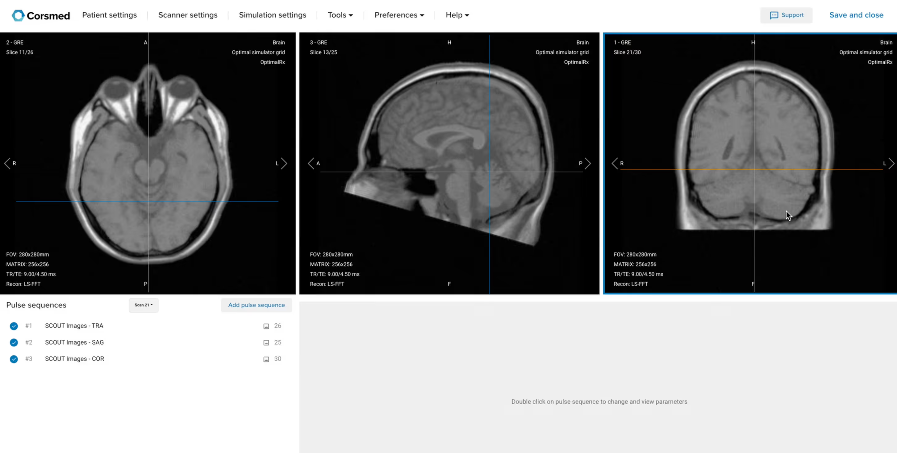
3. Capture the Initial Localizer Images

Before we can perform any MRI protocol, we must always capture initial localizer images of the patient. These images act as a guide for planning the detailed scans we will perform next.

We should always capture localizers in three planes:

1. Axial
2. Sagittal
3. Coronal

Once acquired, upload the initial localizer images into the three viewports.

Then, scroll through each of the image stacks to locate a central slice that clearly shows the anatomy of the brain.

Check that the localizers are aligned and that the head is well-positioned with no rotation. Most importantly, note if there are any previous surgical changes like a craniotomy or a shunt, and check for correct positioning in the isocenter.

✅ Correct Setup of Localizer Images for Brain Tumor MRI:

Part 2: Plan and Acquire the Protocol Sequences

When all preparations are ready, we can start planning and acquiring the protocol sequences.

Let's go through the pulse sequences that a standard brain tumor MRI protocol includes, why we perform them, and how to set them up.

The 5 Pre-Contrast Sequences of a Brain Tumor Protocol (Part 1)

1. Sagittal T1 3D MP-RAGE (Pre-Contrast)
2. Axial T2 TSE
3. Axial T2 FLAIR Fat-Sat
4. Axial Diffusion-Weighted Imaging (DWI) with ADC
5. Axial T2* Gradient Echo

Post-contrast sequences (covered in Part 2):

6. Sagittal T1 3D MP-RAGE (Post-Contrast)
7. Axial T1 TSE (Post-Contrast)
8. Coronal T1 Fat-Sat (Post-Contrast)
9. Axial T1 Fat-Sat (Post-Contrast) – Optional

We mainly use 3D MP-RAGE and Fast/Turbo Spin Echo sequences for this study.

No single sequence provides a complete view on its own. We use 3D MP-RAGE for high-resolution anatomical detail with isotropic voxels, enabling multiplanar reconstruction in any plane. It serves as the baseline for contrast comparison, showing what's naturally bright before gadolinium.

Fast/Turbo Spin Echo sequences let us create multiple contrast weightings (T2, FLAIR) that reveal different tissue properties. T2 shows tumor composition and edema, while FLAIR suppresses CSF to reveal infiltrative margins that extend beyond what other sequences show.

We also use Diffusion-Weighted Imaging to assess tumor cellularity and T2* Gradient Echo to detect hemorrhagic components. Each sequence reveals different aspects of the tumor that together provide a complete picture for diagnosis.

In the sections below, we go through how to plan and set up each pre-contrast sequence.

1. Planning Sagittal T1 3D MP-RAGE (Pre-Contrast)

✅ Correct Planning:

Planning Instructions:

• Use the mid-sagittal line as the anatomical reference.
• Align the slices as follows:
  • Axial Localizer: Parallel to the mid-sagittal line.
  • Coronal Localizer: Parallel to the mid-sagittal line running from the sagittal sinus through the third ventricle to the base of the skull.
• Use appropriate geometry parameters:
  • Slice number: 128 or more to fully cover the brain from side to side with isotropic resolution.
  • Slice thickness: 1–1.2 mm for isotropic voxels, providing equal resolution in all planes for multiplanar reconstruction.
  • Slice gap: 0 mm (contiguous slices) for 3D acquisition.
• Set the fold-over direction (phase encoding) to anterior-posterior (AP) to keep the smallest field of view and reduce scan time.

Parameters for Sagittal T1 3D MP-RAGE:

2. Planning Axial T2 TSE

✅ Correct Planning:

Planning Instructions:

• Use the corpus callosum as the anatomical reference.
• Align the slices as follows:
  • Sagittal Localizer: Parallel to the anterior commissure-posterior commissure (AC-PC) line, or aligned using the genu (front) and splenium (back) of the corpus callosum.
  • Coronal Localizer: Perpendicular to the mid-sagittal line, running from the sagittal sinus through the third ventricle to the base of the skull.
• Use appropriate geometry parameters:
  • Slice number: 30–35 to cover from the vertex to the foramen magnum.
  • Slice thickness: 3–4 mm, slightly thinner than routine brain for better tumor detail.
  • Slice gap: 0–1 mm, minimal gap provides continuity while avoiding cross-talk.
• Set the fold-over direction (phase encoding) to right-left (RL) to reduce wrap-around artifacts and optimize FOV for brain shape.

Parameters for Axial T2 TSE:

3. Planning Axial T2 FLAIR Fat-Sat

✅ Correct Planning:

Planning Instructions:

• Copy the slice geometry and planning from the axial T2 TSE sequence.
• Keep the same slice angulation, coverage, and positioning to ensure images of different contrasts can be clearly compared.

Parameters for Axial T2 FLAIR Fat-Sat:

4. Planning Axial Diffusion-Weighted Imaging (DWI) with ADC Map

✅ Correct Planning:

Planning Instructions:

• Use the corpus callosum as the anatomical reference.
• Align the slices as follows:
  • Sagittal Localizer: Use the same axial prescription as T2/FLAIR, but position the slice package slightly upward and rotate clockwise to avoid paranasal sinuses and oral cavity. Including these air-filled areas causes susceptibility artifacts.
  • Coronal Localizer: Perpendicular to the mid-sagittal line.
• Use appropriate geometry parameters:
  • Slice number: 25–30 to cover the brain while avoiding air-tissue interfaces inferiorly.
  • Slice thickness: 3–4 mm to match other axial sequences when possible.
  • Slice gap: 0–1 mm to maintain continuity between slices.
• Set the fold-over direction (phase encoding) to right-left (RL) to contain geometric distortions to RL direction rather than diagnostically critical AP axis.
• Activate fat suppression (spectral-based), which is required for DWI.
• Set b-values to 0 and 1,000 s/mm² for standard tumor assessment.
• Turn ADC map output to ON to quantify water diffusion and differentiate tumor cellularity.

Parameters for Axial DWI with ADC Map:

5. Planning Axial T2* Gradient Echo

✅ Correct Planning:

Planning Instructions:

• Copy the slice geometry and planning from the axial T2 TSE sequence.
• Keep the same slice angulation, coverage, and positioning to ensure images of different contrasts can be clearly compared.

Parameters for Axial T2* Gradient Echo:

How to Avoid Artifacts When Planning the Sequences

The table below lists the 7 common brain tumor artifacts, and what techniques you can use to avoid them:

Finally, we will review the images to ensure all the anatomical information we need is clear.

These key structures must be clearly visible in a brain tumor MRI:

1. Tumor location, margins, and extent
2. Mass effect and structural distortion
3. Ventricular compression or shift
4. Relationship to eloquent cortex and major vessels
5. Internal tumor composition (solid versus cystic)
6. Edema and infiltrative margins
7. Enhancement patterns

Below, we will go through all the different image contrasts and explain their specific role in imaging brain tumors.

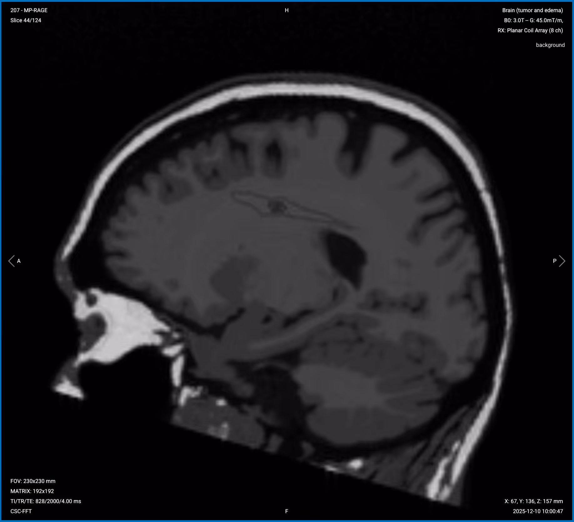
T1 3D MP-RAGE (Pre-Contrast) – Baseline Reference and Anatomical Detail

T1-weighted imaging makes fat appear bright and fluid dark. This contrast is ideal for fat-rich tissues and structural abnormalities. T1 shows anatomical structures clearly, since it helps us see where different solid tissues like muscle and fat meet.

The 3D MP-RAGE sequence uses gradient echo with inversion recovery to optimize tissue contrast.

In brain tumor imaging, pre-contrast T1 3D MP-RAGE serves as the baseline for anatomical assessment. It helps us identify the tumor's location, morphology, and any intrinsic T1 hyperintensity such as hemorrhage, melanin, fat, or protein. It also shows mass effect and structural distortion caused by the tumor, including ventricular compression or midline shift. The thin 1 mm slices enable multiplanar reconstructions in any plane for detailed surgical planning.

We acquire this sequence in the sagittal plane because it provides the most efficient coverage of the entire brain with the smallest field of view, reducing scan time while maintaining isotropic resolution for multiplanar reconstruction.

✅ Sagittal T1 3D MP-RAGE (Pre-Contrast) of the Brain – Correct Image Example:

Things to Look for in Sagittal T1 3D MP-RAGE (Pre-Contrast):

• Entire anatomy of the brain, scrolling through all slices systematically.
• Tumor location and relationship to surrounding structures.
• Intrinsic T1 hyperintensity from hemorrhage, melanin, fat, or protein within the tumor.
• Mass effect and structural distortion around the mass.
• Ventricular compression or shift from the tumor swelling within the skull.

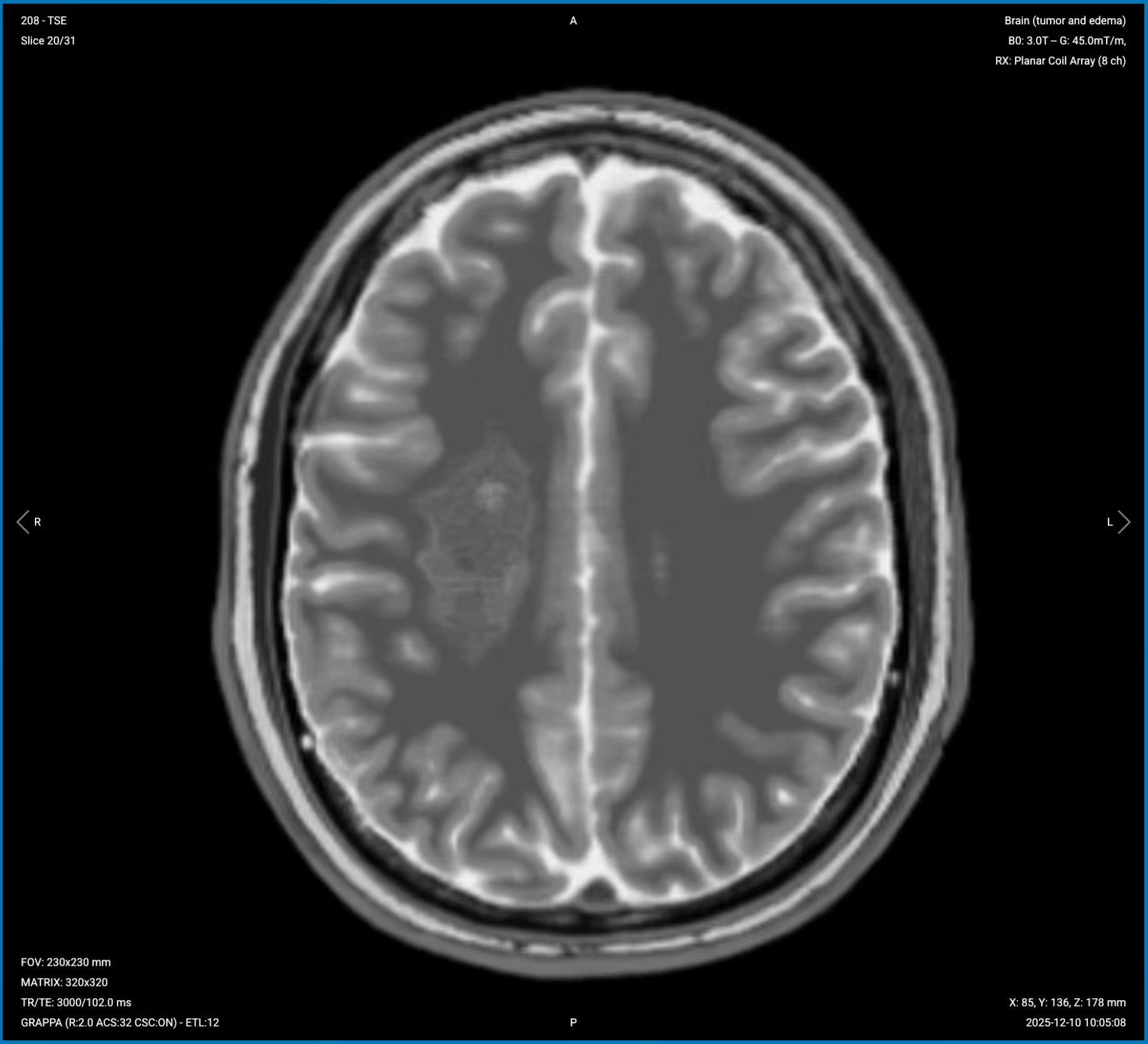
T2 TSE – Shows Tumor Internal Composition and Edema

T2-weighted imaging makes fluids appear bright. This contrast is ideal for tissues and abnormalities with high water content.

In brain tumor imaging, T2 sequences enable us to tell apart cystic and solid components. We can assess the internal architecture and identify edema. For example, a nucleus with liquid hyperintensity on T2 may have a capsule with lower intensity around it. This helps distinguish areas of edema from infiltration and different tumor consistencies.

We acquire this sequence in the axial plane because it provides the best view for assessing left-right symmetry, tumor composition, and mass effect on midline structures and ventricles.

✅ Axial T2 TSE of the Brain – Correct Image Example:

Things to Look for in Axial T2 TSE:

• Tumor composition – cystic areas (bright) versus solid components (lower signal).
• Internal architecture – capsules, multiple compartments, or uniform structure.
• Vasogenic edema surrounding the lesion, appearing bright.
• Mass effect on ventricles, sulci, and midline structures.

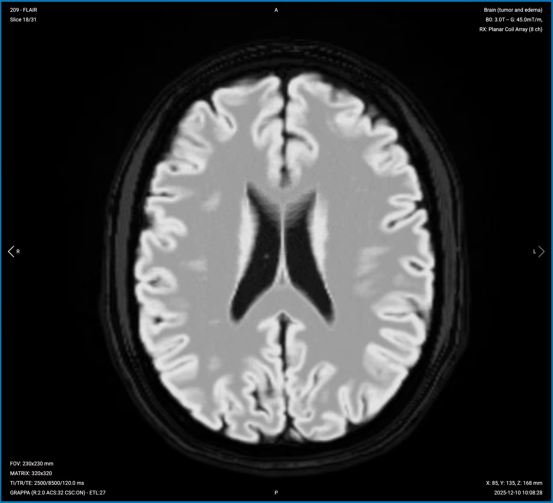
T2 FLAIR Fat-Sat – Best for Infiltrative Margins and Non-Enhancing Tumor Extent

T2 FLAIR (Fluid Attenuated Inversion Recovery) suppresses CSF signal while preserving sensitivity to pathological water. This makes tumor-related abnormalities highly visible, especially near ventricles where bright CSF on standard T2 could obscure lesions.

In brain tumor imaging, FLAIR is critical for detecting infiltrative margins and non-enhancing tumor extension. If the signal doesn't suppress, it's tumor with different timing than CSF, helping us see areas beyond what T2 and post-contrast T1 show. It gives us an intuition of the periventricular situation, whether the tumor infiltrates into the ventricle or not. FLAIR also highlights lesions by suppressing the bright CSF background.

We acquire this sequence in the axial plane to match the T2 TSE, allowing direct comparison between sequences and assessment of infiltrative extent in the same anatomical plane.

✅ Axial T2 FLAIR Fat-Sat of the Brain – Correct Image Example:

Things to Look for in Axial T2 FLAIR Fat-Sat:

• Non-enhancing tumor extent beyond the enhancing margins seen on post-contrast images.
• Infiltrative margins extending into white matter.
• Tumor-related edema clearly visible against dark CSF background.
• Periventricular involvement – check if tumor infiltrates ventricles.
• CSF suppression quality – CSF should appear uniformly dark.

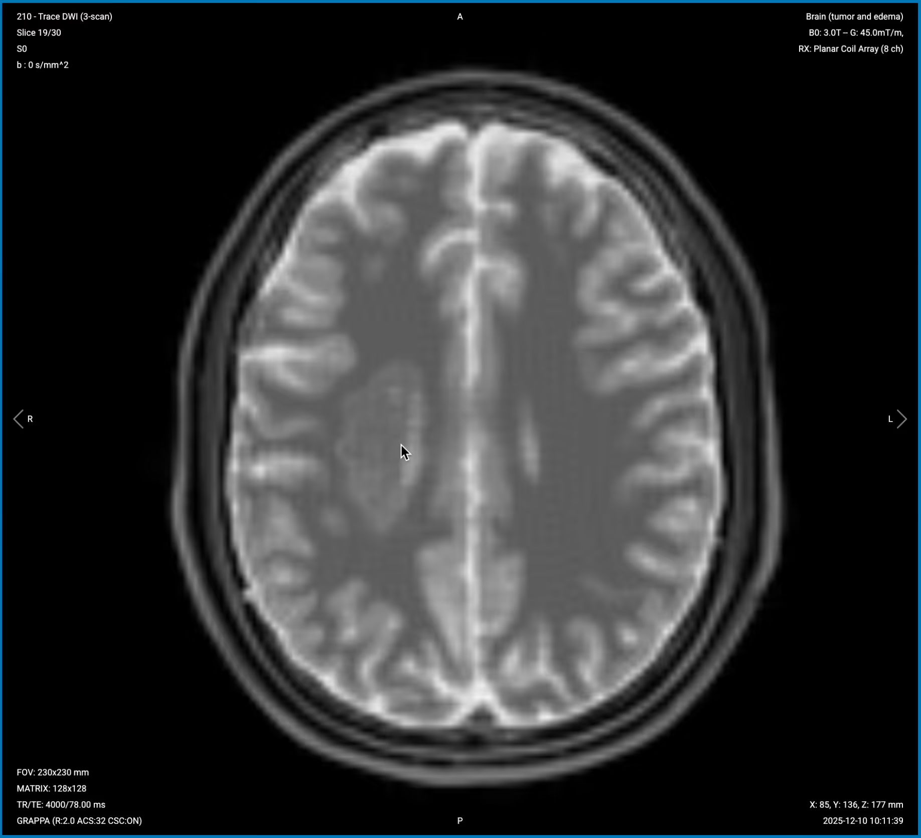
Diffusion-Weighted Imaging (DWI) with ADC – Assesses Tumor Cellularity

Diffusion-weighted imaging detects restricted water molecule movement in tissue. High cellularity restricts diffusion, causing bright signal on DWI and dark signal on ADC maps.

In brain tumor imaging, DWI helps assess tumor cellularity and differentiate between lesion types.

• High diffusion signal and low ADC indicates restricted diffusion, or high cellularity. This can be a sign of high-grade gliomas, lymphomas, or abscesses.
• Low diffusion signal and high ADC indicates facilitated diffusion, or low cellularity. This can be a sign of necrosis, cystic components, vasogenic edema, or low-grade lesions.

This sequence is crucial for distinguishing high-grade gliomas and lymphomas from low-grade tumors, cysts, or necrotic areas. DWI also helps differentiate abscesses (which restrict diffusion) from cystic tumors (which don't).

We acquire this sequence in the axial plane to match other sequences, though with modified coverage to avoid air-tissue interfaces at the skull base that cause severe susceptibility artifacts.

The DWI sequence generates 3 types of images from a single acquisition:

1. b=0 Image (Baseline)

The b=0 image shows tissue without diffusion weighting, essentially a T2-weighted image that serves as an anatomical reference.

✅ Correct Image Example:

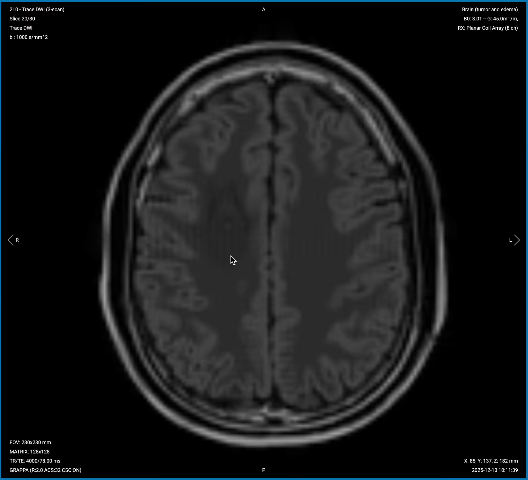
2. True Diffusion Image (b=1000)

The true diffusion image shows areas of restricted water diffusion as bright signal. Select the slice where the tumor is visible to assess diffusion characteristics.

✅ Correct Image Example:

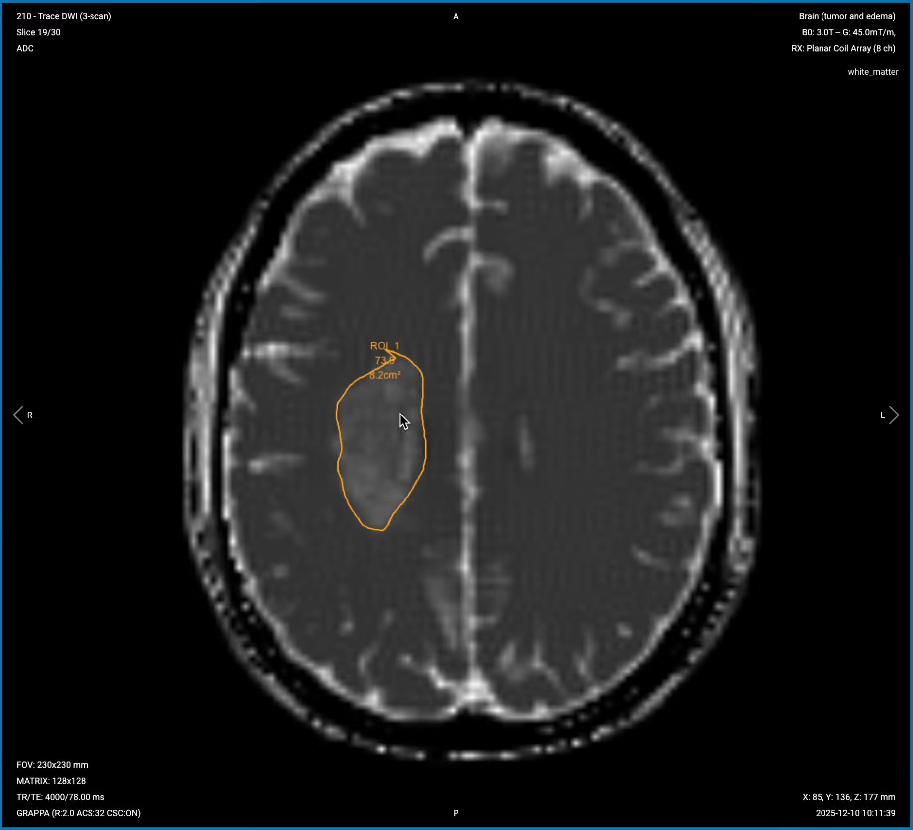
3. ADC Map (Apparent Diffusion Coefficient)

The ADC map quantifies diffusion, where restricted diffusion appears dark and facilitated diffusion appears bright. This confirms whether bright or dark areas on DWI represent true restriction or facilitation.

✅ Correct Image Example:

Things to Look for in DWI and ADC:

• High DWI signal + Low ADC = Restricted diffusion = High cellularity (glioma, lymphoma, abscess).
• Low DWI signal + High ADC = Facilitated diffusion = Low cellularity (necrosis, cystic components, edema, low-grade lesions).
• Diffusion pattern across the mass – uniform or heterogeneous.
• Agreement between DWI and ADC – they should show opposite patterns for true restriction or facilitation.

T2* Gradient Echo – Detects Hemorrhagic Components

T2* gradient echo is highly sensitive to magnetic susceptibility effects from blood products. Hemosiderin, deoxyhemoglobin, and other blood breakdown products cause marked signal loss, appearing as dark blooming artifacts.

In brain tumor imaging, T2* sequences help detect hemorrhagic components and calcification. Look for blooming artifacts or the dual rim sign to confirm hemorrhage or cavernoma. If there's distortion from susceptibility, it could indicate calcification or oligodendroglioma.

We acquire this sequence in the axial plane to match other sequences and allow direct comparison of hemorrhagic findings with tumor margins seen on other contrasts.

✅ Axial T2* Gradient Echo of the Brain – Correct Image Example:

Things to Look for in T2* Gradient Echo:

• Blooming artifacts from blood products appearing as dark signal.
• Dual rim sign indicating specific types of hemorrhage.
• Susceptibility distortion that might indicate calcification.
• Microhemorrhages within or around the tumor.

Final Checks

Before finishing the pre-contrast portion of a brain tumor MRI, always check these 6 points to ensure diagnostic quality:

1. Complete Coverage: All sequences must cover from vertex to foramen magnum, including the entire lesion and surrounding edema.
2. Isotropic Resolution on T1 3D : The T1 3D MP-RAGE must have isotropic voxels (1–1.2 mm³) for multiplanar reconstruction.
3. Matching Axial Prescriptions: All axial sequences (T2, FLAIR, DWI, T2*) must have matching slice positions for direct comparison.
4. CSF Suppression on FLAIR: CSF in ventricles must appear dark on FLAIR; bright CSF indicates inadequate suppression.
5. DWI and ADC Agreement: High cellularity lesions must show bright DWI with dark ADC. Low cellularity must show low DWI with high ADC.
6. Image Quality: All sequences must have adequate SNR, minimal motion artifacts, and appropriate resolution for tumor margins.

This completes Part 1 of the brain tumor MRI protocol, covering all pre-contrast sequences.

In Part 2, we will cover:

• Contrast injection timing and technique
• Post-contrast sagittal T1 3D MP-RAGE
• Post-contrast axial and coronal T1 sequences
• Post-contrast T1 with fat suppression
• Complete image review and diagnostic principles
• Final protocol checklist

The pre-contrast sequences we've acquired provide important baseline information about tumor composition, cellularity, and extent. The post-contrast sequences in Part 2 will reveal blood-brain barrier breakdown and help characterize tumor vascularity and aggressiveness.

‍