How to plan a brain tumor MRI protocol (part 2: post-contrast)

This step-by-step guide is for MRI students, radiographers, and technologists who wish to improve their planning skills and master the brain tumor MRI protocol.

This guide is Part 2 of planning a brain tumor MRI assessment. In Part 1, we covered pre-contrast imaging and tumor characterization.

In this Part 2, we will follow up with contrast injection and post-contrast imaging, where we identify enhancement patterns that guide tumor diagnosis and treatment planning.

What you will learn:

1. Key factors in brain tumor MRIs, including trade-offs.
2. How to perform the contrast injection workflow.
3. Best post-contrast pulse sequences and planning techniques.
4. Ways to avoid common artifacts.
5. Qualities of great brain tumor images.

In Part 1 of our brain tumor protocol, we completed all pre-contrast sequences. We captured baseline anatomical information with 3D MP-RAGE, assessed tumor composition with T2 and FLAIR, evaluated cellularity with diffusion-weighted imaging, and checked for hemorrhage with T2* gradient echo.

Now we continue with another core part of brain tumor assessment: contrast-enhanced imaging. This is where we identify enhancement patterns that guide diagnosis and treatment planning.

Enhancement patterns narrow the differential. They do not settle it, and the radiologist makes the call.

• Rim enhancement: raises high-grade glioma, abscess, or metastasis
• Homogeneous enhancement: raises meningioma, lymphoma, or some metastases
• Nodular enhancement: raises hemangioblastoma or a complex cystic lesion
• No enhancement: raises low-grade glioma, though some high-grade gliomas enhance minimally

These patterns directly impact treatment decisions and prognosis.

How to Balance the 3 Trade-offs in Brain Tumor MRIs

In MRI, we always face a trade-off between 3 key metrics:

• Scan Time: How fast a pulse sequence can be completed.
• Resolution: How much detail the image can display.
• SNR: How clear the image is, meaning how much signal we have compared with noise.

Improving one of these metrics often reduces the performance of the others. To decide what trade-offs to make, we must consider the needs of each clinical situation.

For brain tumor MRIs, we face these challenges:

• Missing a 2 mm metastasis could change treatment entirely. We need to see small lesions clearly and detect infiltrative margins that extend into normal brain tissue.
• We must differentiate between different tumor types based on their signal characteristics. This requires adequate image clarity to distinguish subtle differences in tissue properties.
• Brain tumor protocols are comprehensive studies that include many sequences. Most patients can tolerate around 30 minutes of scanning, but beyond that, motion artifacts can make images completely unreadable.

Therefore, we typically:

1. Prioritize resolution to detect small metastases and infiltrative margins,
2. Keep good SNR to ensure adequate image clarity for our resolution targets, and
3. Optimize scan time as needed to stay within the practical limit of around 30 minutes.

Post-Contrast Brain Tumor Conditions and the MRI Sequences That Reveal Them

These are some of the most common brain tumor conditions we look for in post-contrast imaging, and which pulse sequences reveal them:

The Contrast Injection Workflow

The whole workflow hinges on one rule: plan every post-contrast sequence before the contrast goes in. Anything left unplanned costs enhancement window.

For Manual Injection:

1. Insert cannula in patient's arm
2. Position patient at isocenter
3. Acquire all pre-contrast sequences
4. Plan all post-contrast sequences
5. Slide patient table out of bore
6. Enter scan room with prepared syringe
7. Inject contrast slowly through cannula
8. Press isocenter button to reposition patient
9. Return to control room and start post-contrast acquisitions 5 minutes after starting the injection

For Automated Power Injection:

1. Insert cannula in patient's arm
2. Connect IV line from injector to cannula
3. Position patient at isocenter
4. Acquire all pre-contrast sequences
5. Plan all post-contrast sequences
6. Set injection parameters (volume, flow rate, etc.)
7. Initiate injection from control room
8. Wait 5 minutes after starting the injection, then start post-contrast sequences

In both workflows, planning post-contrast sequences happens before contrast injection (Step 4 in the manual workflow, Step 5 in the automated workflow).

How to Perform Brain Tumor Contrast-Enhanced Imaging

The step-by-step guide below will show you how to perform contrast-enhanced imaging for brain tumor assessment, the second part of a complete brain tumor protocol.

In Part 1, we set up the patient, captured localizer images, and acquired all pre-contrast sequences. Now in Part 2, we will perform the protocol in 3 steps:

1. Plan and Set Up the Post-Contrast Sequences
2. Inject the Contrast Agent
3. Review the Images

Step 1: Plan and Set Up the Post-Contrast Sequences

Before we inject contrast, we must plan all post-contrast sequences and have them ready to run. This ensures we don’t waste any time after injection.

The 3 post-contrast sequences of a standard brain tumor MRI protocol:

1. Sagittal T1 3D MP-RAGE
2. Axial T1 TSE Fat-Sat (Post-Contrast)
3. Coronal T1 TSE Fat-Sat (Post-Contrast)

We use T1-weighted sequences after contrast because they show enhancement patterns that guide diagnosis.

A matched isotropic 3D T1 acquisition is central to post-contrast tumor imaging, and MP-RAGE is the sequence used here. The fat-suppressed T1 TSE sequences confirm enhancement patterns and remove fat signal that could obscure pathology.

In the sections below, we go through how to plan and set up each sequence.

1. Planning Sagittal T1 3D MP-RAGE (Post-Contrast)

✅ Correct Planning:

Planning Instructions:

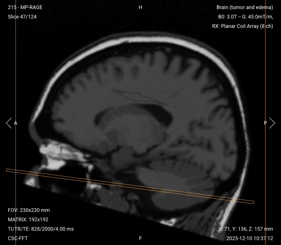
• Copy the slice geometry and planning from the pre-contrast sagittal T1 3D MP-RAGE sequence.
• Keep the same slice angulation, coverage, and positioning to ensure precise comparison between pre- and post-contrast images.
• Use identical spatial resolution and planning to enable side-by-side overlay comparison.

Parameters for Post-Contrast Sagittal T1 3D MP-RAGE:

Use the same parameters as the pre-contrast T1 3D MP-RAGE sequence, with one exception: parallel imaging is added here to keep the acquisition inside the enhancement window, which the pre-contrast sequence has no need to race against.

This is a 3D acquisition, so slices are contiguous, with no gap between them.

2. Planning Axial T1 TSE Fat-Sat (Post-Contrast)

✅ Correct Planning:

Planning Instructions:

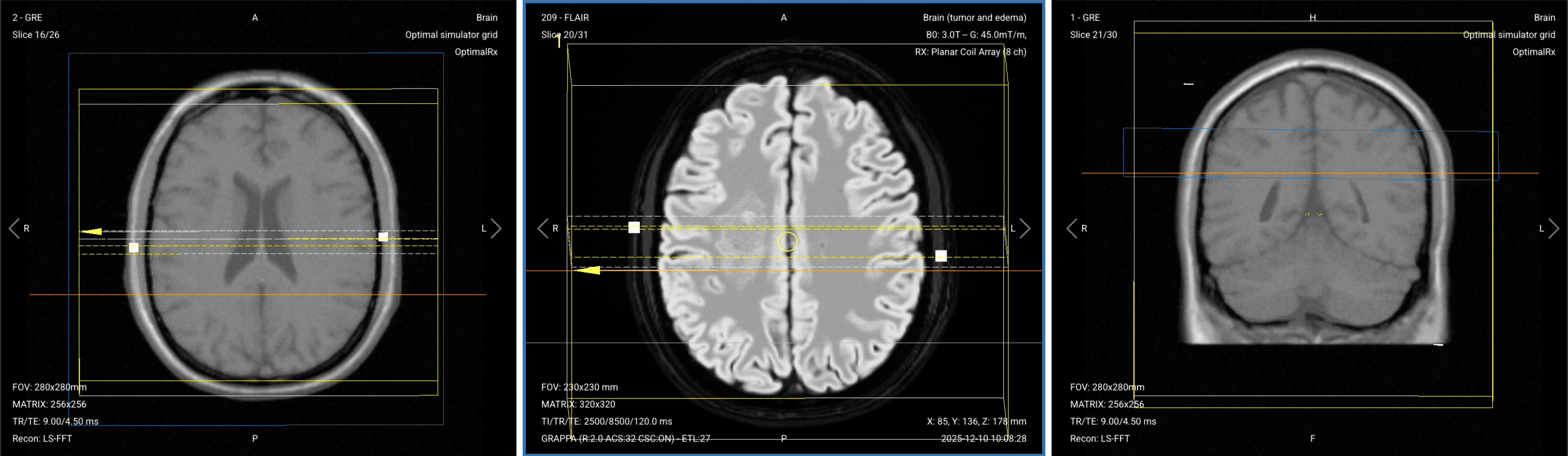
• Copy the slice geometry and planning from the axial T2 TSE sequence.
• Keep the same slice angulation, coverage, and positioning to ensure images can be easily compared with other axial sequences.
• Acquire this sequence directly after the 3D completes.

Parameters for Post-Contrast Axial T1 TSE Fat-Sat:

3. Planning Coronal T1 TSE Fat-Sat (Post-Contrast)

✅ Correct Planning:

Planning Instructions:

• Use the post-contrast sagittal T1 3D MP-RAGE for planning.
• Align the slices as follows:
  • Sagittal Localizer: Perpendicular to the midsagittal line of the brain.
  • Axial Localizer: Ensure slices run from anterior (frontal lobe) to posterior (occipital lobe) without cutting out any anatomy.
• Use appropriate geometry parameters:
  • Slice number: Enough to cover from the posterior fossa to the frontal lobe (typically 30–35 slices).
  • Slice thickness: 4 mm, medium thickness for good resolution without sacrificing scan time or SNR.
  • Slice gap: 1 mm, 25% of slice thickness, which limits cross-talk without hiding anatomy.
• Set the fold-over direction (phase encoding) to right-left (RL) to minimize wraparound artifacts and allow the smallest field of view.
• Acquire this sequence directly after the axial completes. Enhancement is weaker by this point, and fat suppression contributes more to the clarity of this sequence than the exact timing does.

Parameters for Post-Contrast Coronal T1 TSE Fat-Sat:

How to Avoid Artifacts When Planning the Sequences

The table below lists the 6 artifacts that affect the post-contrast sequences, and what techniques you can use to avoid them. See Part 1 for diffusion-related geometric distortion.

Step 2: Inject the Contrast Agent

Now that all post-contrast sequences are planned and ready, we proceed with contrast injection following the workflow outlined earlier.

1. Verify Patient Safety

Before any contrast injection, you must verify that the patient can handle it. Contrast safety follows local policy and the agent in use. For patients with acute kidney injury or an eGFR below 30 mL/min/1.73 m², the decision weighs the benefit of the study against the agent's risk group, and it belongs to the radiologist rather than the radiographer. A standard dose of a modern macrocyclic agent carries very low risk even at low eGFR, so a needed study should not be cancelled reflexively. Check the local cutoff and approval route before the patient arrives.

If contrast cannot be given safely, complete and report the pre-contrast series and discuss the case with the radiologist before ending the exam. Never compromise patient safety for imaging.

2. Contrast Dosing

The dose is prescribed in millimoles per kilogram, not in milliliters. The standard adult dose for brain imaging is 0.1 mmol/kg.

Convert to a volume using the concentration printed on the vial in front of you:

Volume (mL) = 0.1 mmol/kg × weight (kg) ÷ concentration (mmol/mL)

For an 80 kg patient the dose is 8 mmol, which gives:

Never carry a milliliter figure across from another site or another agent. Recalculate from the concentration on the vial every time.

3. Timing Protocol

After the injection, follow this order:

1. Wait 5 minutes from the start of the injection, so the contrast distributes into the tissue and the vessel signal fades.
2. Start the 3D MP-RAGE. It takes roughly 6 minutes.
3. Run the axial T1 with fat suppression directly after it completes. It takes roughly 6 minutes.
4. Run the coronal T1 directly after the axial completes.

Whichever delay your department uses before the first post-contrast sequence, use the same delay for every follow-up study, so the images stay comparable.

Finally, we will review the images to ensure all the anatomical information we need is clear.

These key structures must be clearly visible in a brain tumor MRI:

1. Tumor location, margins, and extent
2. Mass effect and structural distortion
3. Ventricular compression or shift
4. Relationship to eloquent cortex and major vessels
5. Internal tumor composition (solid versus cystic)
6. Edema and infiltrative margins
7. Enhancement patterns

Below, we will go through all the different image contrasts and explain their specific role in imaging brain tumors.

Post-Contrast T1 3D MP-RAGE – Reveals Enhancement Patterns

A matched isotropic 3D T1 acquisition is central to post-contrast tumor imaging, and MP-RAGE is the sequence used here for detecting tumor enhancement and abnormal blood-brain barrier breakdown.

In brain tumor imaging, post-contrast T1 3D MP-RAGE reveals enhancement patterns that guide diagnosis and tumor grading. Rim enhancement with a central hypointense core suggests high-grade glioma, abscess, or metastasis. Homogeneous enhancement indicates meningioma, lymphoma, or some metastases.

Absence of enhancement suggests low-grade glioma, though some high-grade gliomas also show minimal enhancement. Nodular enhancement appears in hemangioblastomas and some cystic lesions. The thin 1.2 mm slices allow detection of subtle enhancement and enable multiplanar reconstructions for detailed assessment.

We acquire this sequence in sagittal orientation because it provides volumetric coverage that can be reconstructed in any plane while maintaining isotropic resolution.

✅ Sagittal T1 3D MP-RAGE (Post-Contrast) – Correct Image Example:

Things to Look for in Post-Contrast T1 3D MP-RAGE:

• Enhancement pattern (rim, homogeneous, nodular, or absent)
• Dural tail sign suggesting meningioma
• Vascular encasement or invasion
• Small enhancing foci scattered through the parenchyma, which can indicate metastases, lymphoma, or infection
• Compare carefully with pre-contrast T1 to distinguish true enhancement from intrinsic T1 hyperintensity

Post-Contrast Axial T1 TSE Fat-Sat – Confirms Enhancement Patterns

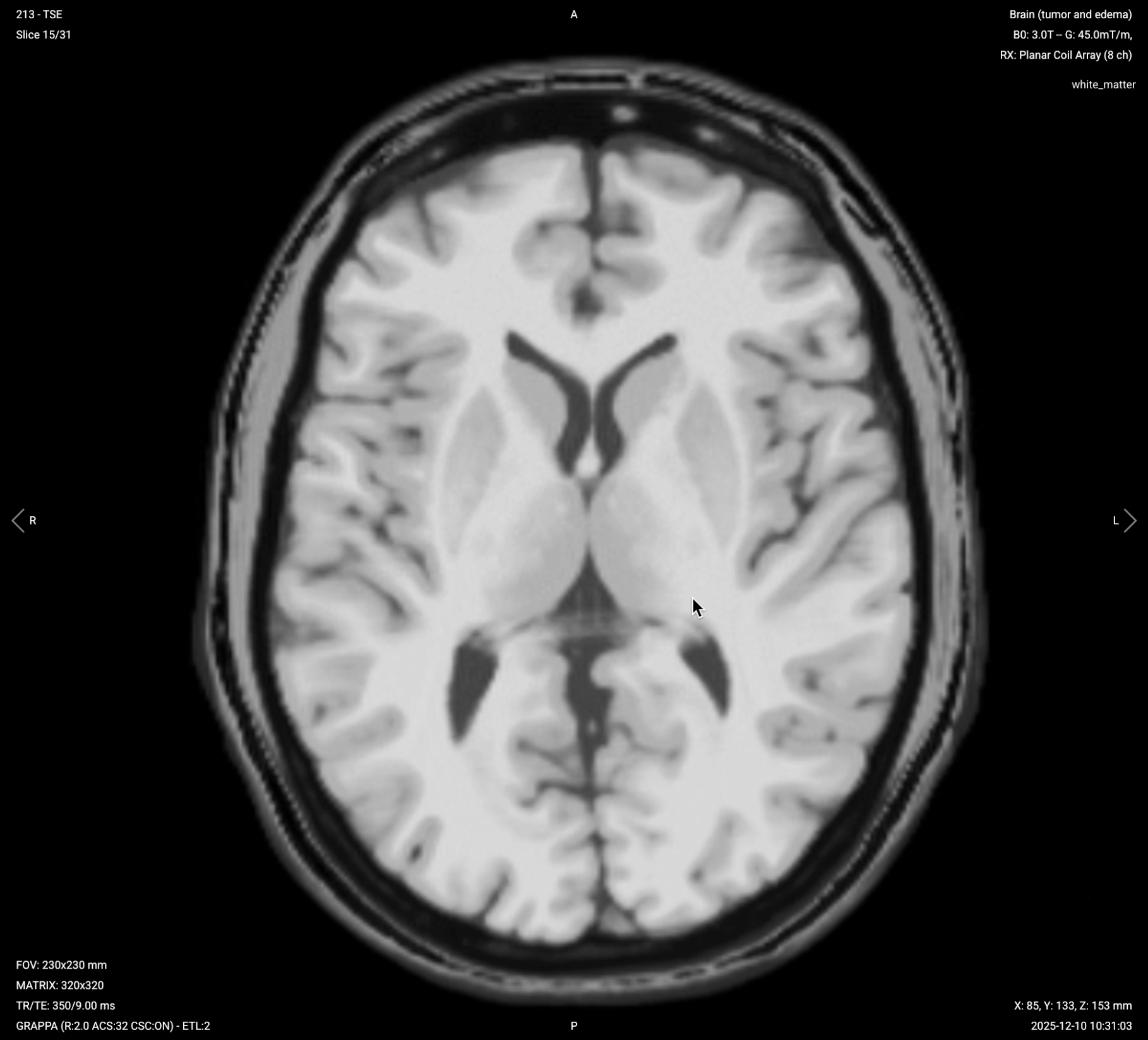
Post-contrast T1 with fat suppression reduces bright signal from fat, making true contrast enhancement stand out more clearly.

In brain tumor imaging, axial post-contrast T1 with fat suppression confirms enhancement patterns seen on the 3D MP-RAGE from a different angle. Fat suppression removes bright fat signal so enhancement near the skull base and in extra-axial tumors is not masked. It does not separate enhancement from hemorrhage, which the matched pre-contrast and post-contrast T1 images show instead. This sequence is acquired directly after the 3D, while parenchymal enhancement is still strong, making subtle tumor enhancement more visible.

We acquire this sequence in axial orientation to match other standard axial sequences and enable direct comparison with pre-contrast images.

✅ Axial T1 with Fat Suppression (Post-Contrast) – Correct Image Example:

Things to Look for in Post-Contrast Axial T1 with Fat Suppression:

• Confirmation of enhancement patterns from different angle
• Subtle enhancement that may be obscured by fat without suppression
• Clear distinction between enhancement and fat, with the pre-contrast T1 used to rule out intrinsic T1 hyperintensity from blood
• Relationship of enhancing tumor to surrounding structures
• Absence of fat signal near skull base clarifying true enhancement

Post-Contrast Coronal T1 TSE Fat-Sat – Assesses Superior-Inferior Extent

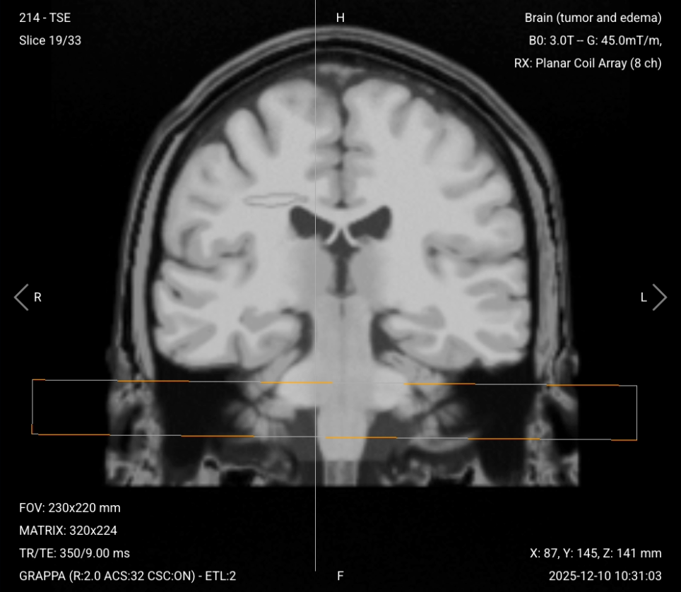
Post-contrast coronal T1 with fat suppression provides a frontal perspective of tumor enhancement with fat signal suppressed.

In brain tumor imaging, coronal post-contrast T1 with fat suppression assesses the superior-inferior extent of the tumor and its enhancement. This view is particularly useful for identifying dural involvement, meningeal spread, and skull base invasion. Fat suppression clarifies enhancement along the meninges and skull base where fat might otherwise obscure pathology. This sequence complements the sagittal and axial post-contrast images for complete three-dimensional assessment.

We acquire this sequence in coronal orientation to complete the three orthogonal planes and provide optimal assessment of superior-inferior tumor relationships.

✅ Coronal T1 with Fat Suppression (Post-Contrast) – Correct Image Example:

Things to Look for in Post-Contrast Coronal T1 with Fat Suppression:

• Superior-inferior tumor extent and enhancement
• Dural involvement or meningeal spread along brain surface
• Skull base invasion
• Relationship to cranial nerves and vascular structures

Final Checks

Before finishing a post-contrast brain tumor MRI, always check these 6 points to ensure diagnostic quality:

1. Pre- and Post-Contrast Comparison: Pre-contrast and post-contrast T1 images must have identical planning to enable accurate comparison and enhancement assessment.
2. Complete Coverage: All sequences must fully cover the entire tumor and surrounding brain tissue, with no anatomical structures cut off.
3. Enhancement Pattern Clarity: Post-contrast images must clearly show enhancement patterns, with the post-contrast series started after the department's standard delay, and the same delay used for every follow-up study.
4. Multiplanar Assessment: Tumor must be evaluated in all three planes (axial, sagittal, coronal) for complete spatial understanding.
5. Fat Suppression Quality: Post-contrast sequences with fat suppression must show uniform fat suppression, making true enhancement clearly visible.
6. Image Quality and Artifacts: Images must have strong SNR, crisp detail, and minimal motion, chemical shift, susceptibility, or wrap-around artifacts. Motion artifacts matter most in brain tumor protocols, because the study runs long.

‍